Getting started with Google Earth Engine

Learning Objectives
Access your code editor
Create your own repository, folders and files
Basic JavaScript syntax
Find and import datasets in the code editor
Create variables from known coordinates
Visualise geometries
Find and import online GEE datasets
Images
Visualise images
Images with multiple bands
Feature collections
Filtering feature collections
Image collections filtered by dates and bands
Simple functions and single images
Simple functions and image collections
Sharing your code to complete the practical assignments
Complete code example

Author: Sandra MacFadyen

Access complete code on Google Earth Engine

Learning Objectives

By the end of this practical you should be able to:

Understand the basic layout of Google Earth Engine platform (incl. the Code Editor).
Understand basic JavaScript syntax rules.
Find and import datasets into the code editor.
Inspect a dataset in the console.
Visualize datasets in the interactive map explorer.
Use simple functions.
Know where to find help.

Access your code editor

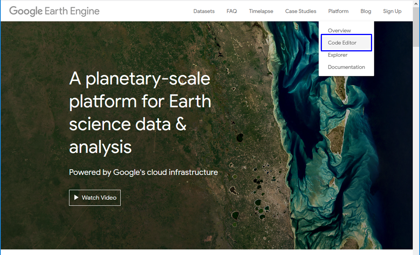
The first step is to access the GEE code editor. This can be done from the earth engine home page by going to platform –> Code Editor. Alternatively, you can access it directly from https://code.earthengine.google.com/

gee_screenshot1

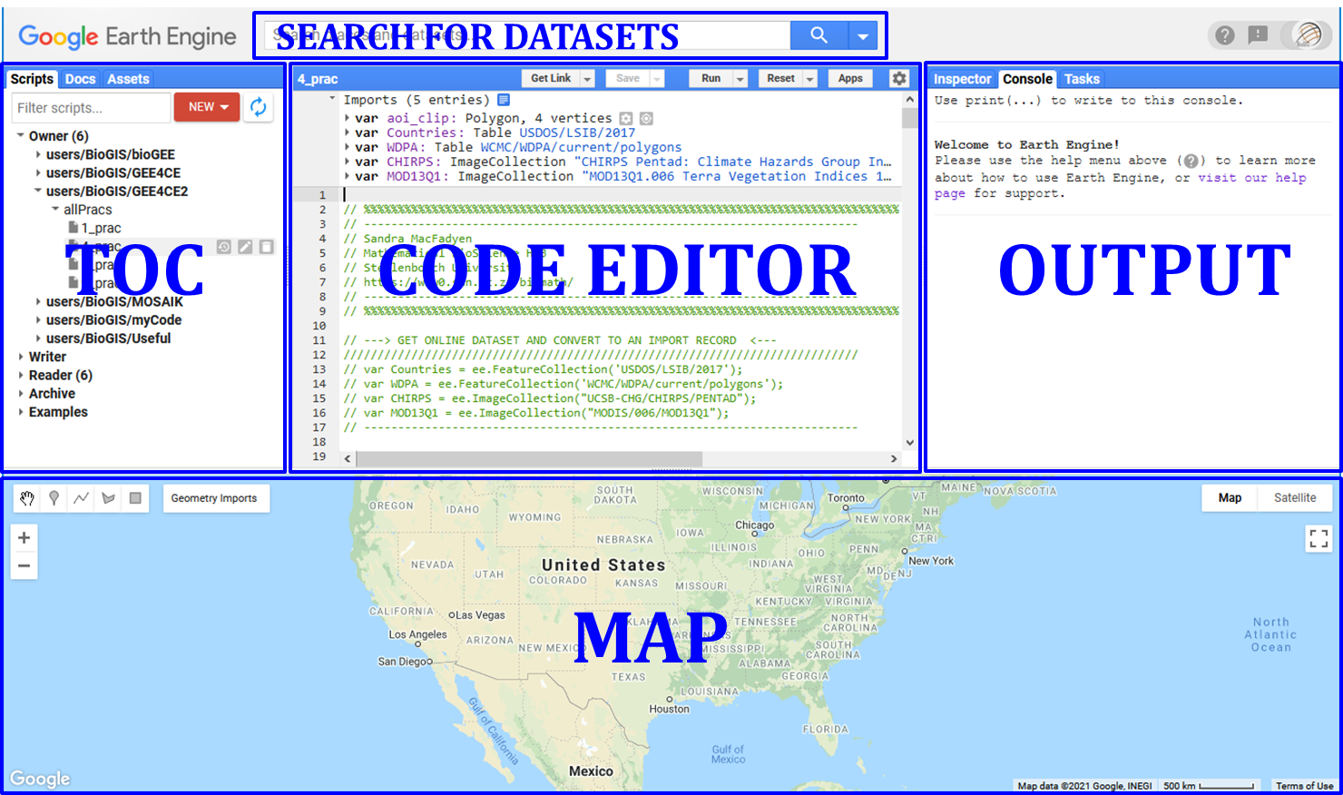
Take a look at the Google Earth Engine » Guides » Earth Engine Code Editor section for a nice description of different panels and tabs.

gee_screenshot2

Create your own repository, folders and files

From the Scripts panel click NEW » Repository or » Folder or » File. Or if you already have a script open, click Save » Save as..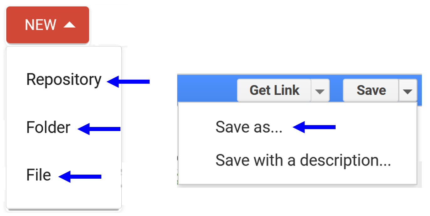 gee_screenshot3

Basic JavaScript syntax

Let’s start off with a simple “Hello World” exercise:

print('Welcome to the world of GEE!');
var myMessage = 'GEE world - Sandra was here :)'; // Variable or object
print(myMessage);

Find and import datasets in the code editor

Draw your own

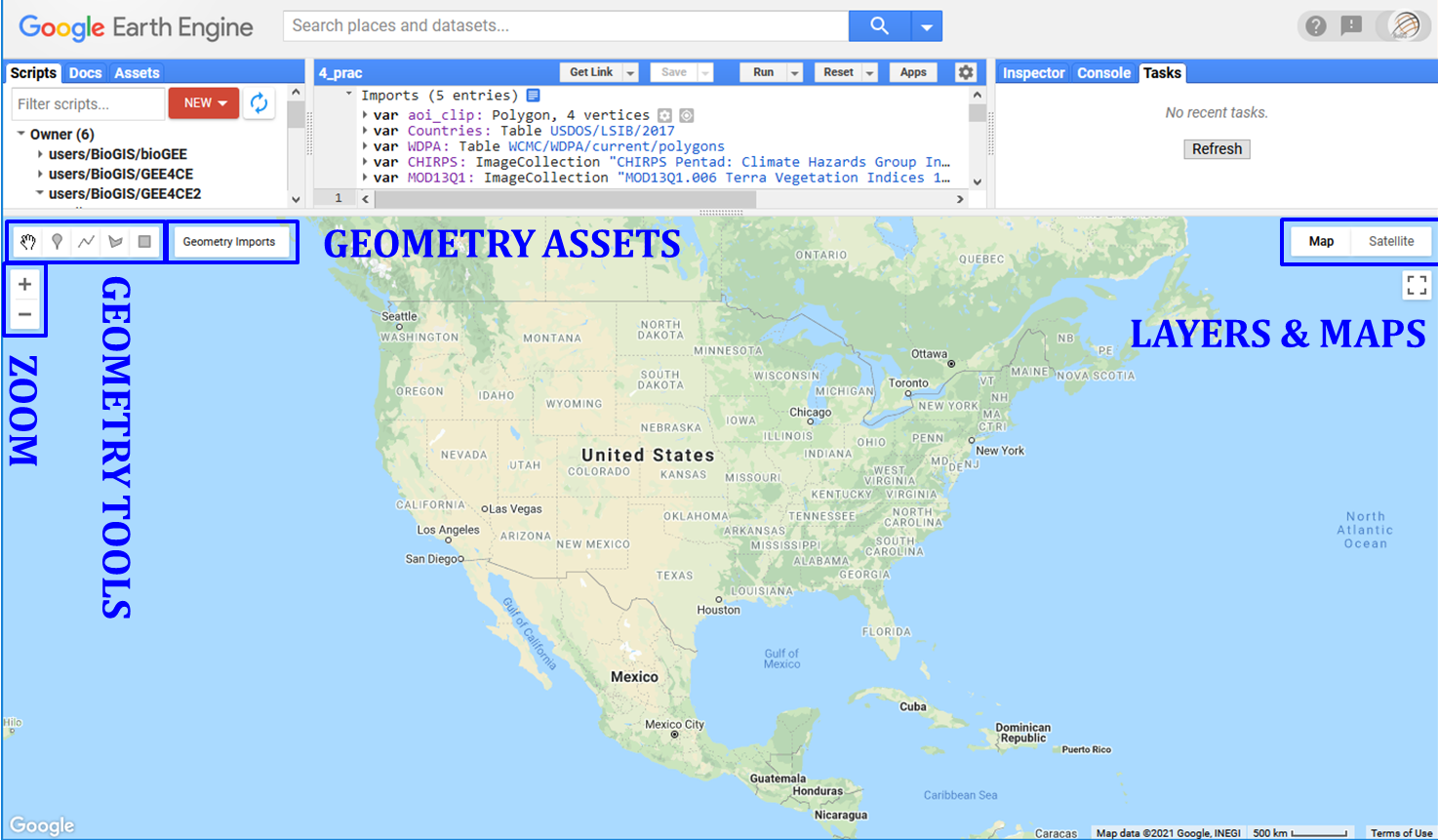
Create your first import variables using the geometry tools. For example, “Add a marker” or “Draw a rectangle”. See the new ‘geometry’ variable added to the ‘Imports’ section? You can ‘Edit layer properties’ e.g. the name or colour from “Geometry Import” or assets. It is important to ‘Exit’ the ‘Point drawing’ and ‘+ new layer’ to avoid creating a ‘GeometryCollection’ instead of a ‘Point’ geometry.

gee_screenshot3

Create variables from known coordinates

Or you can create your own variables using known coordinates.

var skukuza = ee.Geometry.Point([31.5912, -24.9947]);
var krugerAOI = ee.Geometry.Polygon([[[30.6821, -22.2315], [30.6821, -25.5061], 
                                      [32.1542, -25.5061], [32.1542, -22.2315]]]);</code><button class="btn" id="copy-button" data-clipboard-target="#target2">Copy</button>

Visualise geometries

To display these new variables on the map area below, you need to use the Map. commands. First zoom to a location on the map and then add the new variable as a layer with user defined display/legend properties.

// First center and zoom to a location on the map
// There are different ways to center your map
Map.setCenter(31.54, -23.96, 7); // Use the "Inspector" to click and get coords
Map.centerObject(krugerAOI, 7); // Or using your geometry variable

// Then add the variable to the map and change the colours
Map.addLayer(krugerAOI, {color: 'green'}, 'Kruger Park');
Map.addLayer(skukuza, {color: 'red'}, 'Skukuza Camp');</

Find and import online GEE datasets

To find GEE datasets, use the “Search places and datasets” panel visible in the Code Editor or browse datasets by satellite platform or keyword tags from the Earth Engine Catalog page.

Images

To import images from GEE you will use ee.Image(). There are two ways you can do this. The easiest is to use the search function and then click Import to add the dataset to your Imports section.

gee_screenshot3

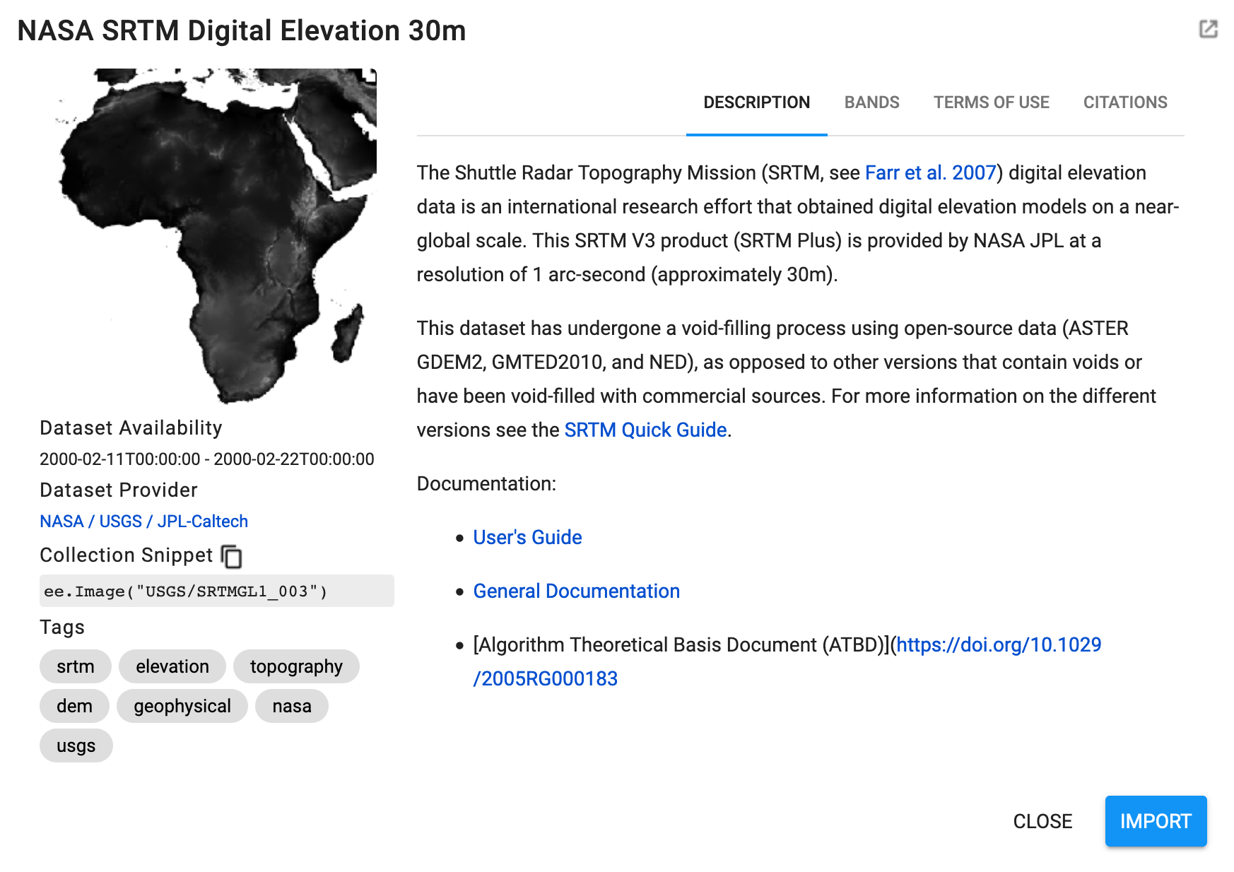
The second is to copy the Collection Snippet code and paste it into your script. Don’t forget to make a new variable to hold the dataset.

var elevation = ee.Image('USGS/SRTMGL1_003');
print('Elevation variable info', elevation); // Print is your friend
print('Elevation data type', elevation.name()); // Prints data type

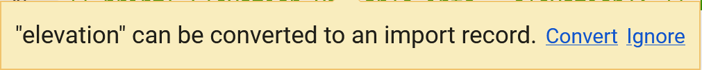
Once you’ve done that, if you hold your mouse over your new variable/code, you’ll see a yellow message pop-up asking if you want to convert it to an import record. If you click Convert, the variable will be moved to the Imports section automatically.

gee_screenshot3

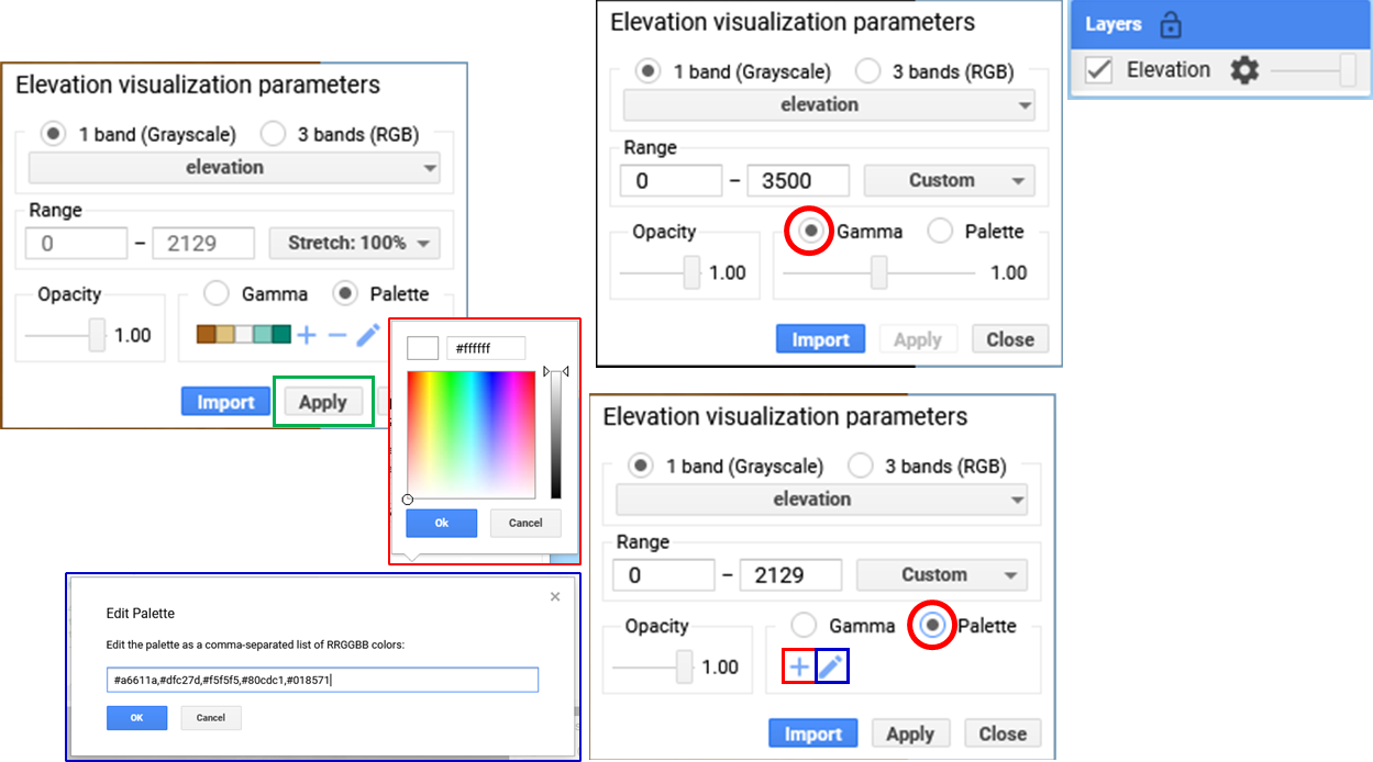
Visualise images

To display images in your map you zoom to a location of interest and add then add the image as a layer but with more detailed display/legend properties. You can do this using the “Visualization Parameters” GUI or code it directly(see code box below).

gee_screenshot3

// Center your map to specific area and zoom level
Map.setCenter(31.54, -23.96, 7);
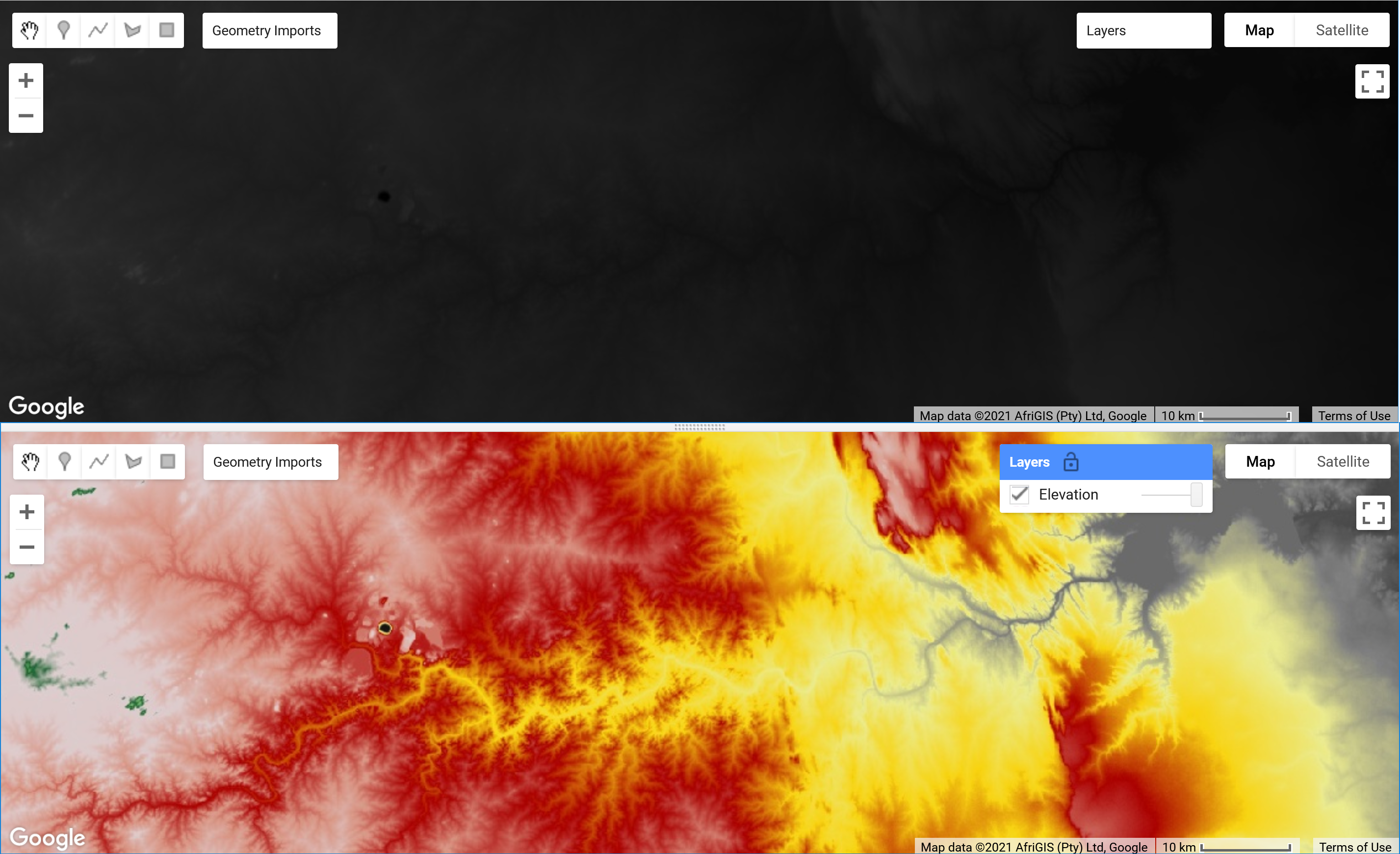
// Play with the legend parameters
Map.addLayer(elevation, {min: 0, max: 3500}, 'Elevation'); // Try without specific colours
Map.addLayer(elevation, {min: 0, max: 3500, palette: ['blue','yellow','red']}, 'Elevation'); // Now add colour range
// !NB! It matters what order you add variables to the map

// What if we need a palette to display the variable better?
var eleVis = {
  min: 0,
  max: 1000,
  palette: [
    '141414', '383838', '808080', 'EBEB8F', 'F7D311', 'AA0000', 'D89382',
    'DDC9C9', 'DCCDCE', '1C6330', '68AA63', 'B5C98E', 'E1F0E5', 'a975ba',
    '6f198c'
  ],
};
// Here are some guides to help you find colours
// e.g. #DAF7A6,#FFC300,#FF5733,#C70039,#900C3F,#581845 
// https://colorbrewer2.org/#type=sequential&scheme=BuGn&n=3
// https://github.com/gee-community/ee-palettes

Map.setCenter(31.54, -23.96, 7);
Map.addLayer(elevation, eleVis, 'Elevation with eleVis'); // See how different your two layers look?

gee_screenshot3

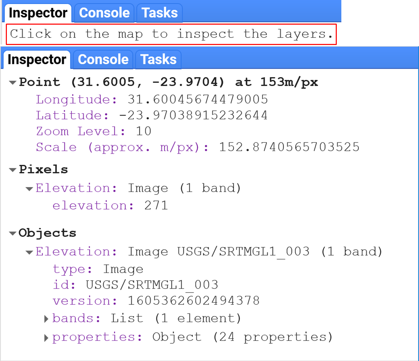
Use the ‘Inspector’ to get “Point”, “Pixel” and “Object” information.

gee_screenshot3

Images with multiple bands

WorldClim BIO Variables V1. Most of you will probably be familiar with WoldClim’s Bioclimatic Variables. There are 19 different variables coded bio01 to bio19 e.g. bio01 = Annual mean

bio02 = Mean diurnal

bio03 = Isothermality (bio02/bio07)

bio04 = Temperature seasonality etc.

gee_screenshot3

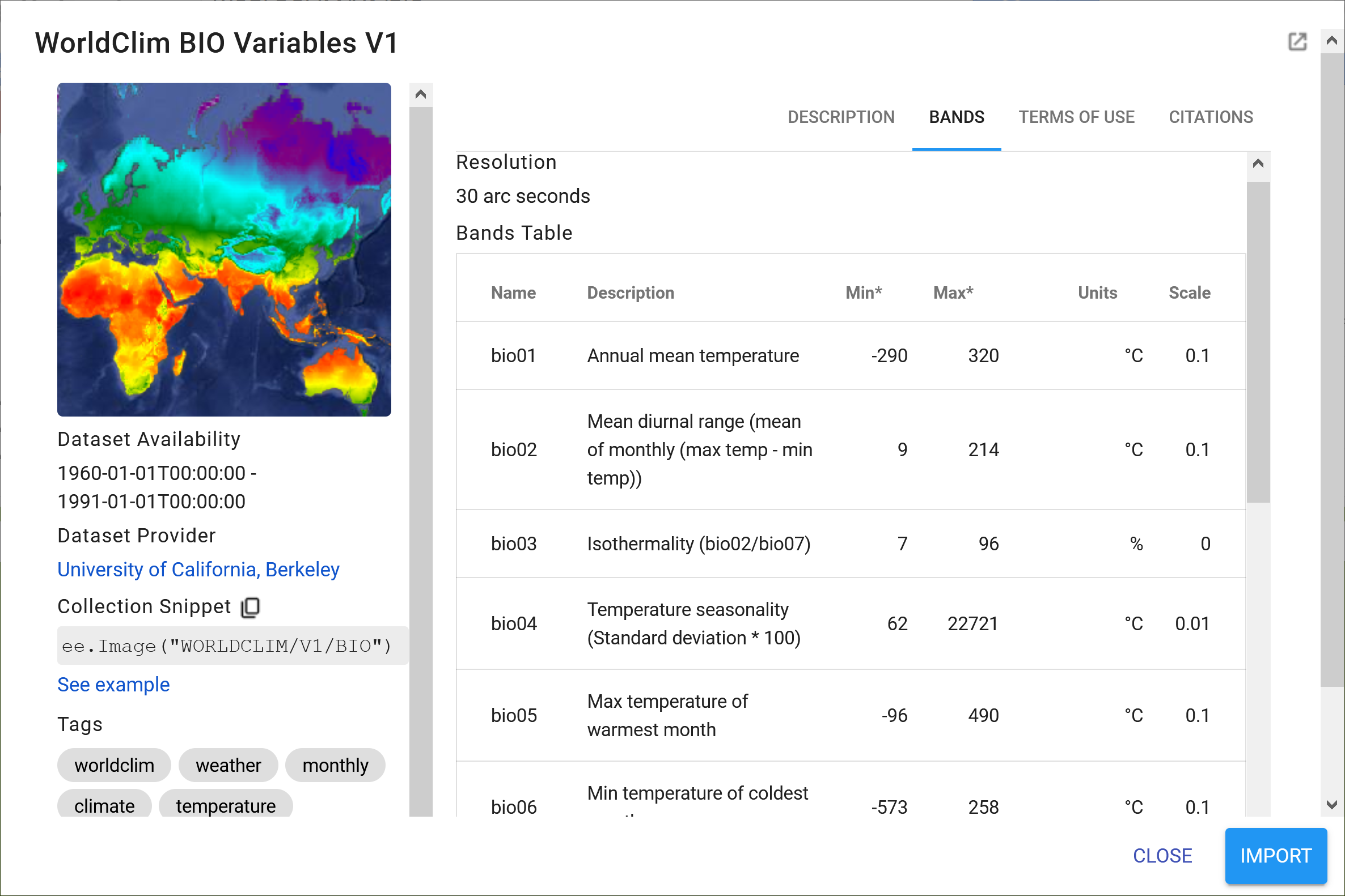
To use one of these variables you need to select the appropriate band. For example “Annual Mean Temperature”.

// Import WorldClim BIO Variables V1
var bio = ee.Image('WORLDCLIM/V1/BIO');
var amt = bio.select('bio01');

// Same thing, less code
// var amt = ee.Image('WORLDCLIM/V1/BIO').select('bio01'); 

// Your display/legend properties
var amtVis = {
  min: -230.0,
  max: 300.0,
  palette: ['blue', 'purple', 'cyan', 'green', 'yellow', 'red'],
};

// Display the results on your map below
Map.setCenter(31.54, -23.96, 2);
Map.centerObject(krugerAOI, 7);
Map.addLayer(amt, amtVis, 'Annual Mean Temperature');
Map.addLayer(krugerAOI, {color: 'green'}, 'Kruger Park');
// !NB! Remember it matters what order you add variables to the map

Feature collections

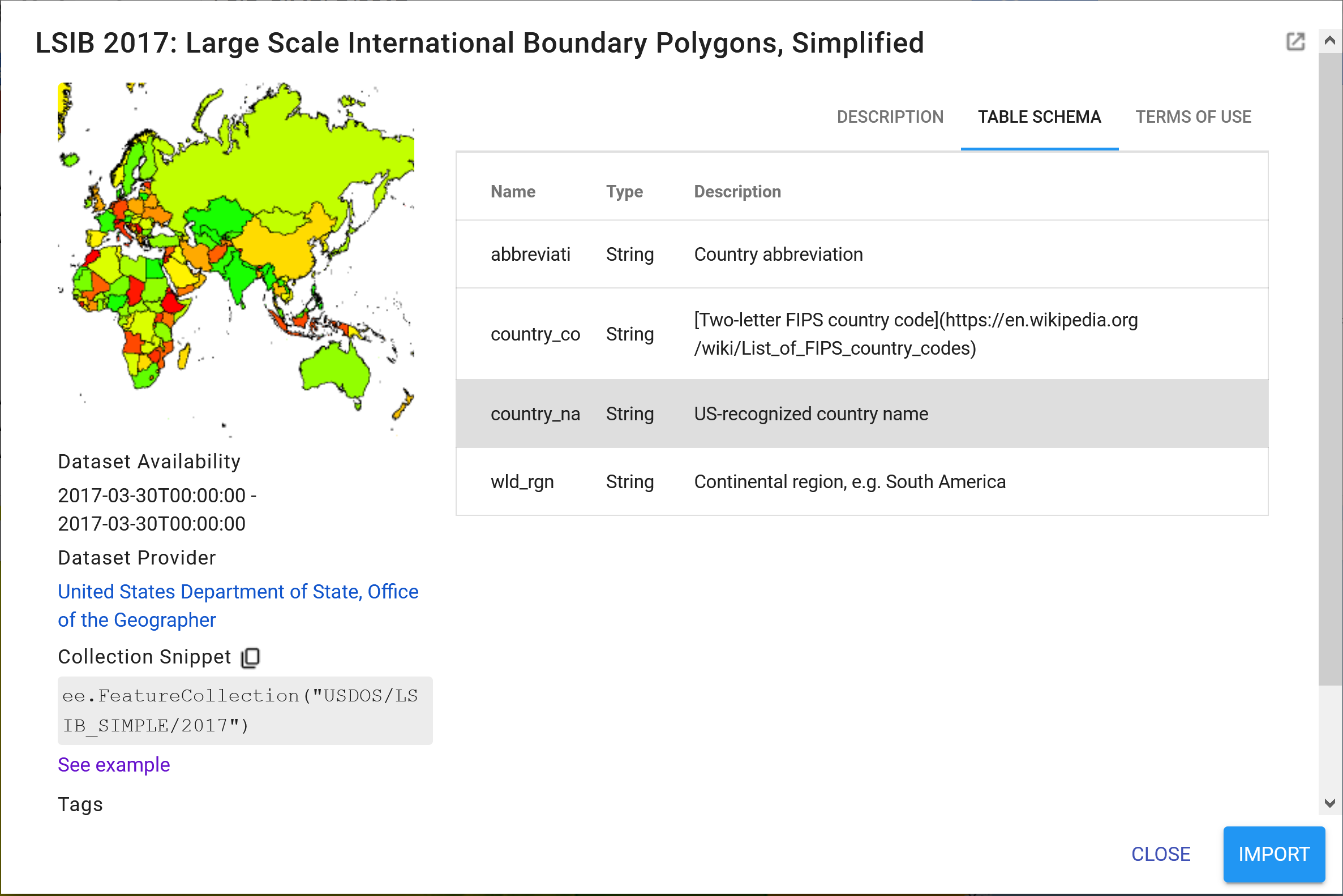
Feature collections work in a similar way to image collections, although the display parameters and filtering conditions are slightly different. For example, let’s display International Boundaries as polygons (i.e. vectors).

gee_screenshot3

// Import the simplified International Boundary Polygons (LSIB 2017) 
var countries = ee.FeatureCollection("USDOS/LSIB_SIMPLE/2017");

// Your display properties
var cntVis = {
    fillColor: 'b5ffb4',
    color: '00909F',
    width: 3.0,
};

// Add results to map
Map.setCenter(23.63, 5.68, 2);
Map.addLayer(countries, cntVis, 'World Borders');

Filtering feature collections

Now to filter the features we need to know what column/field our contains the information we would like to filter for. In this case it’s a “string” field named “country_na” as indicated in the “TABLE SCHEMA” in the figure above.

// Country boundaries filtered to Costa Rica
var costaRica = countries.filter(ee.Filter.eq('country_na', 'Costa Rica'));
print('eq Costa Rica', costaRica); // Remember, this returns info about our feature

// Add results to map
Map.centerObject(costaRica, 7);
Map.addLayer(costaRica,{}, 'Costa Rica');

// Country boundaries filtered to Costa Rica  and Colombia or a "list" of values
var costaColo = countries.filter(ee.Filter.inList('country_na',['Costa Rica','Colombia']));
print('costaColo data type',costaColo.name()); // Returns ComputedObject type
print('inList costaColo', costaColo); // Returns info about feature
Map.centerObject(costaColo, 4);
Map.addLayer(costaColo,{}, 'Costa Rica and Colombia');

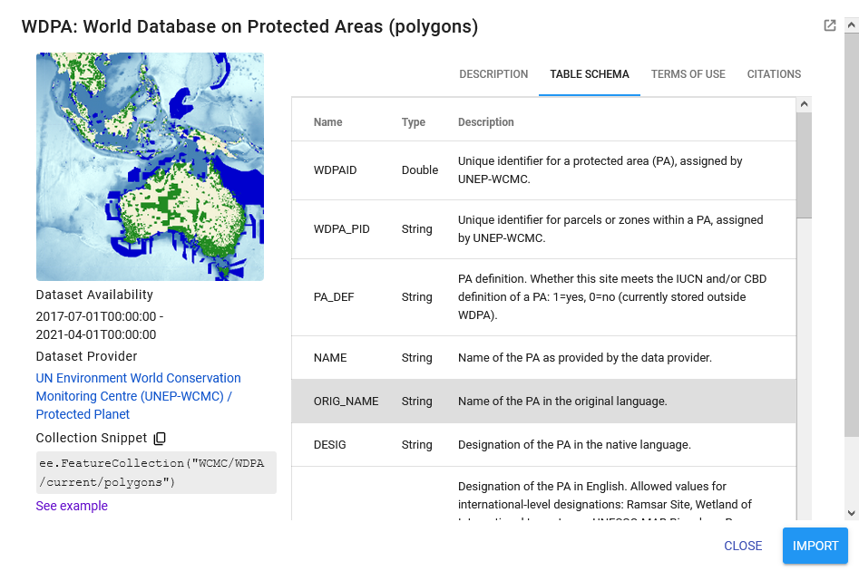
Here is another example using polygons depicting the World Database on Protected Areas (WDPA).

gee_screenshot3

// Import the WDPA polygons
var WDPA = ee.FeatureCollection('WCMC/WDPA/current/polygons');
// WDPA boundaries filtered to 'Kruger' National Park' in South Africa
var kruger = WDPA.filter(ee.Filter.eq('ORIG_NAME', 'Kruger National Park'));
// print('Kruger Info',kruger);

// Add results to map
Map.centerObject(kruger, 7);
Map.addLayer(kruger,{fillColor:'ceea89',color:'789630',width:0.5}, 'Kruger National Park');

Image collections filtered by dates and bands

In many cases you will be dealing with image collections with a series of bands over a period of time. To filter for the date range you’re interested in you will use the ee.Filter.date command. Let’s test this using the 500m monthly burned area product from MODIS.

gee_screenshot3

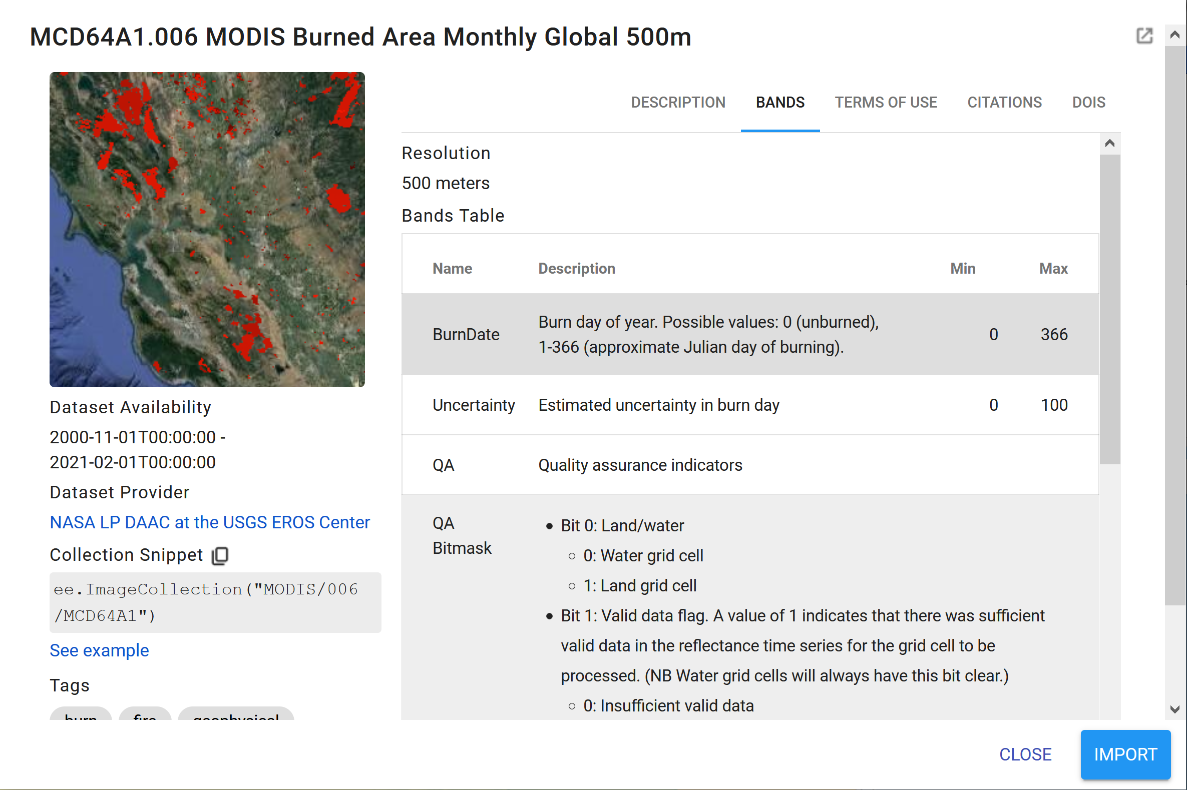
// Import the MODIS Burned Area Monthly Global 500m
var modis64 = ee.ImageCollection('MODIS/006/MCD64A1');
var modisBurn = modis64.select('BurnDate');
var burnArea = modisBurn.filter(ee.Filter.date('2018-01-01', '2018-12-31'));
print('burnArea Info long', burnArea);

// Visual parameters for legend
var burnVis = {
  min: 30.0,
  max: 341.0,
  palette: ['4e0400', '951003', 'c61503', 'ff1901'],
};

// Add results to map
Map.centerObject(krugerAOI, 7);
Map.addLayer(burnArea, burnVis, 'Areas Burnt Oct 2018');

Simple functions and single images

There are many built-in functions you can use to process and analyse the different GEE data products. We will be going through a number of these in our different practical sessions but for now let’s look at some simple ones to get you started. The most common is probably the .clip function, which we’ll test on our elevation data from earlier.

// Clip the elevation data to your area of interest
var eleClip = elevation.clip(costaRica);

// Add results to map
Map.centerObject(costaRica, 7);
Map.addLayer(eleClip, {min: 0, max: 350, palette: ['blue','yellow','red']}, 
                      'Costa Rica Elevation');

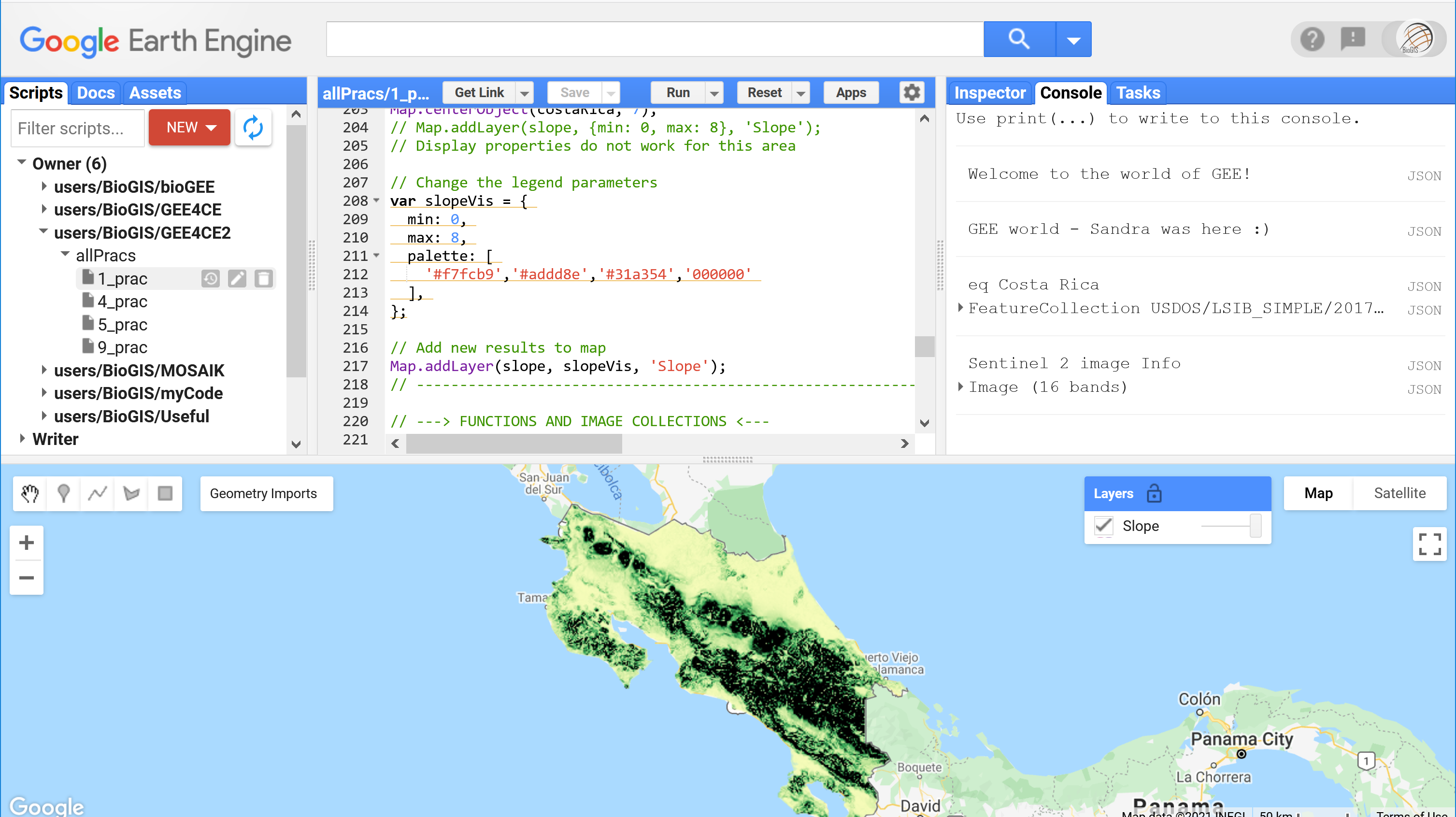
Let’s try generating a slope from this new elevation variable using the built-in ee.Terrain.slope function.

// Generate a slope from the clipped SRTM elevation model
var slope = ee.Terrain.slope(eleClip);

// Add results to map
Map.centerObject(costaRica, 7);
Map.addLayer(slope, {min: 0, max: 8}, 'Slope', false);
// Display properties do not work for this area

// Change the legend parameters 
var slopeVis = {
  min: 0,
  max: 8,
  palette: [
    '#f7fcb9','#addd8e','#31a354','000000'
  ],
};

// Add new results to map
Map.addLayer(slope, slopeVis, 'Slope with palette');

gee_screenshot3

Simple functions and image collections

Applying functions to image collections starts to get a little trickier. For example, let’s try summarise some Sentinel-2 imagery (Sentinel-2 MSI: MultiSpectral Instrument, Level-1C)and change our display properties at the same time.

gee_screenshot3

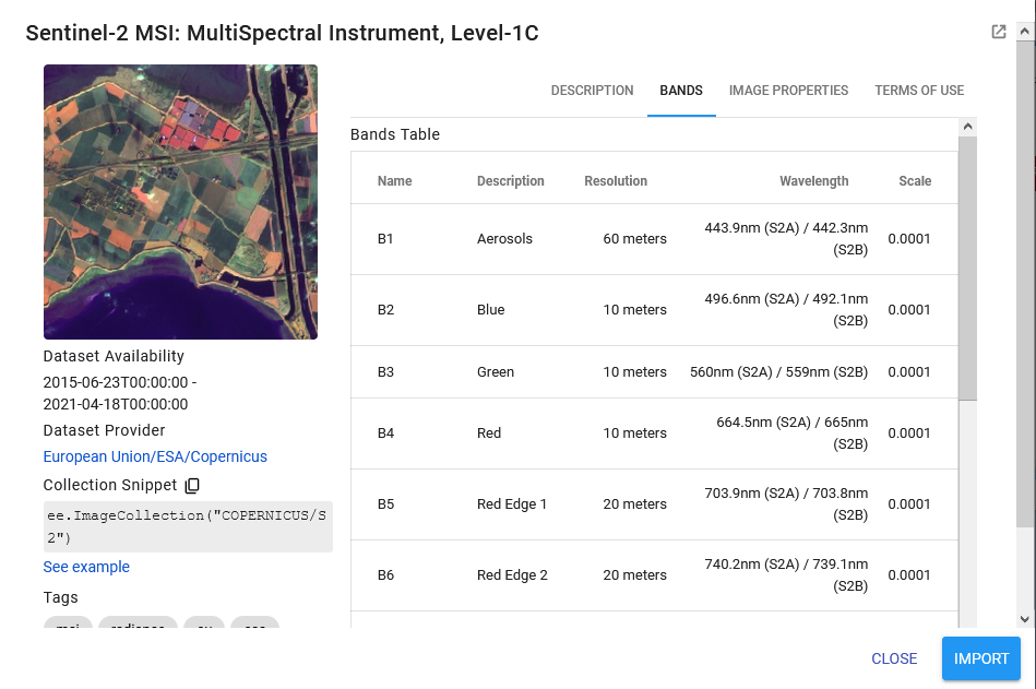
// Import Sentinel-2 imagery
// Filter the image collection based on several properties
var copCol = ee.ImageCollection("COPERNICUS/S2")
               .filter(ee.Filter.date('2018-01-01','2019-12-31')) // Filter date range
               .filterBounds(krugerAOI); // Filter area
print('copCol Info', copCol);

// Calculates a median value for all pixels over this time period                            
var cop2Med =  copCol.median();
// Or you could use *.sort("CLOUD_COVERAGE_ASSESSMENT")*
// And them select the first image of the collection 
// i.e. the most cloud free, using *.first()* instead of .median()

// Check output
print('Sentinel 2 image Info', cop2Med);

// Add new results to map
Map.setCenter(31.5975, -24.9945, 12);
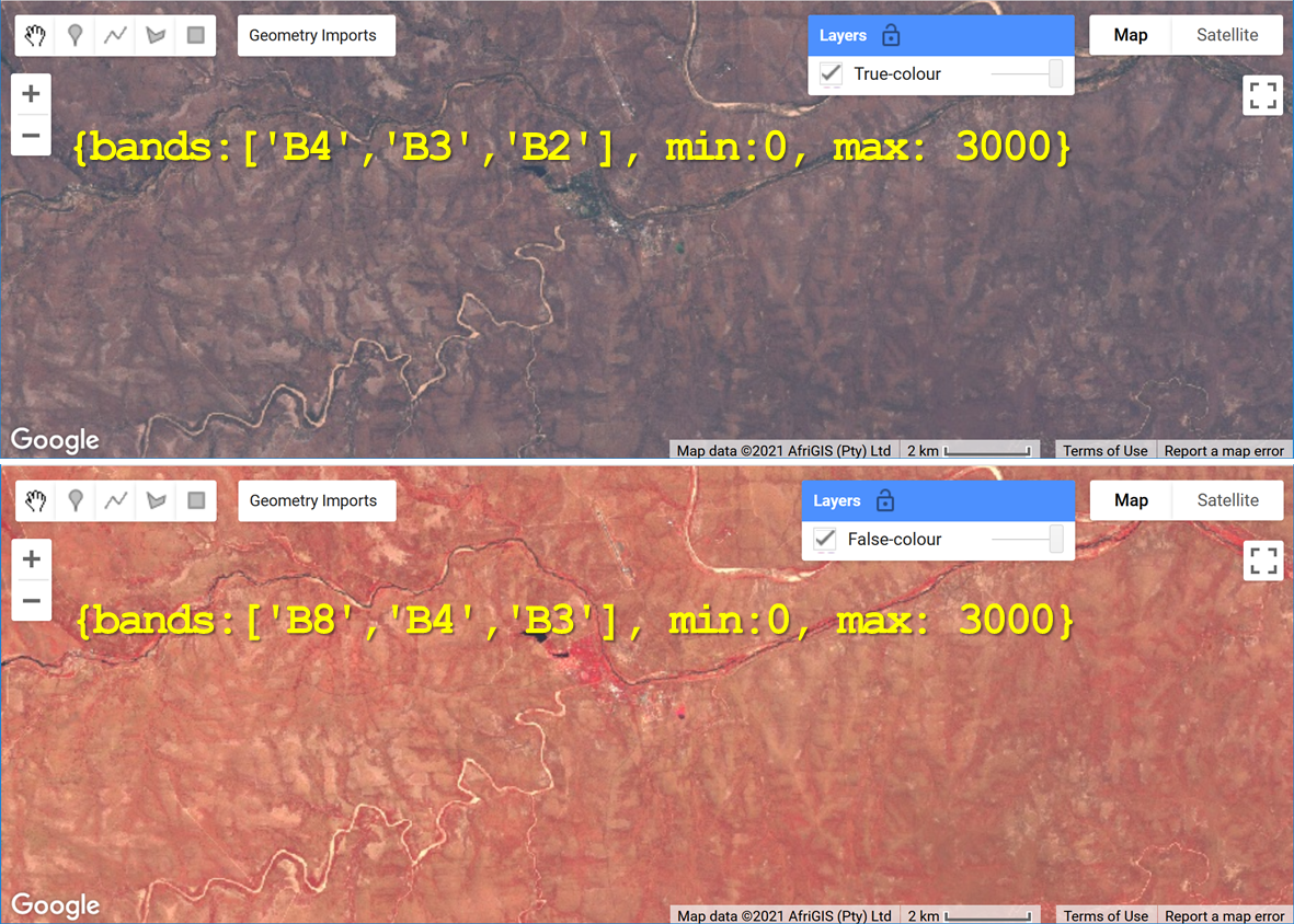
// Select Bands 4, 3 and 2 = red, green and blue bands to make a true-colour composite
// Add this RGB composite to map, without defined parameters
Map.addLayer(cop2Med, {bands:['B4','B3','B2']}, 'No defined vis parameters');
// Results are rubbish

gee_screenshot3

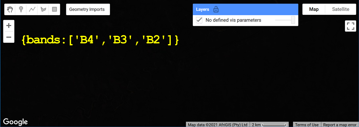
// Add the S2 value range from 0 to 3000, and try again
Map.addLayer(cop2Med, {bands:['B4','B3','B2'], min:0, max: 3000}, 'True-colour');
// You can also change the order of bands e.g. B8,B4,B3 = false-colour composite etc
Map.addLayer(cop2Med, {bands:['B8','B4','B3'], min:0, max: 3000}, 'False-colour');
// Here using the NIR band, this false-colour shows photosynthetically 
// active vegetation in bright red

gee_screenshot3

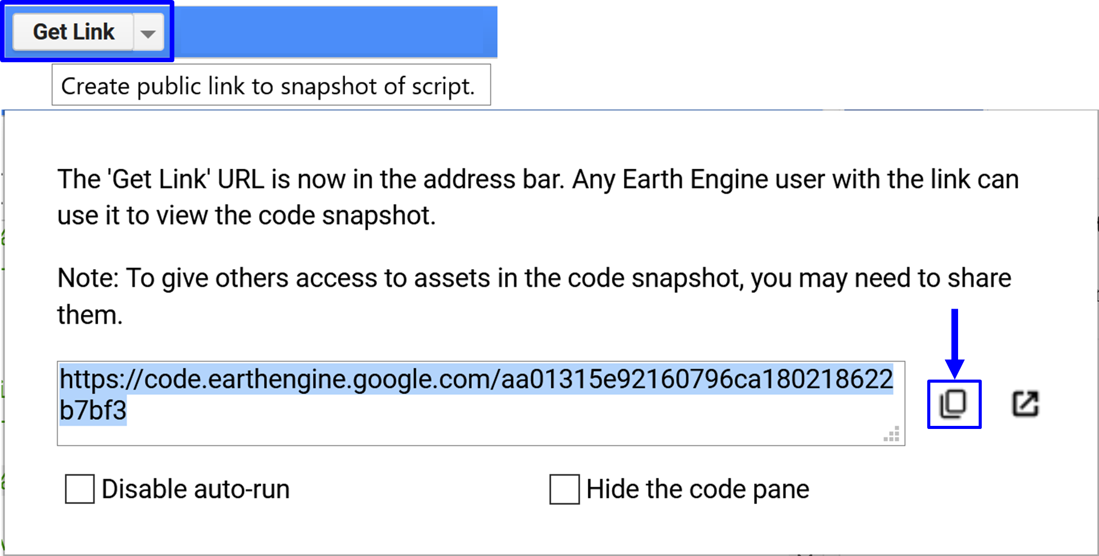
To complete the practical exercise below you need to know how to share your scripts with us. Simply click on “Get Link” - the actual button NOT the dropdown arrow - Then click the “Click to copy link” button and paste that in an email. !NB! Please remember to add the prac number in the header.

gee_screenshot3

Complete code example

// ---> CREATE YOUR OWN REPOSITORY/FOLDER/FILE <---
////////////////////////////////////////////////////////////////////////////
// From the Scripts panel click NEW >> Repository
// In here you can also create separate folders in much the same way
// i.e. Click NEW >> Folder
// When you first open the Code Editor, a New Script should open, 
// waiting for you to start adding your code
// If not, you can create one NEW >> File or click Save >> Save as..
// -------------------------------------------------------------------------
// ---> WELCOME TO THE WORLD OF GEE AND JAVASCRIPT<---
////////////////////////////////////////////////////////////////////////////
// See PowerPoint presentation from this session for more info
print('Welcome to the world of GEE!');
var myMessage = 'GEE world - Sandra was here :)'; // Illustrates variable object
print(myMessage);
// -------------------------------------------------------------------------
// ---> CREATE YOUR FIRST IMPORT VARIABLES USING THE GEOMETRY TOOLS <---
//////////////////////////////////////////////////////////////////////////
// Add a marker ==> See the new 'geometry' variable added to the 'Imports' section?
// You can 'Edit layer properties' e.g. the name or colour
// !NB! 'Exit' the 'Point drawing' and '+ new layer' to avoid making a 'GeometryCollection' instead of a 'Point'

// Now 'Draw a rectangle' 
// '+ new layer', draw your rectangle then 'Edit layer properties'
// See how these new variables show up as layers under 'Geometry Imports'
// -------------------------------------------------------------------------
// ---> CREATE VARIABLES USING KNOWN COORDINATES - ADDED TO LAYERS <---
////////////////////////////////////////////////////////////////////////////
// You can create your own variables from coordinates
var skukuza = ee.Geometry.Point([31.5912, -24.9947]);
var krugerAOI = ee.Geometry.Polygon([[[30.6821, -22.2315], [30.6821, -25.5061], 
                                      [32.1542, -25.5061], [32.1542, -22.2315]]]);

// How do you display them on the map though?
// First center and zoom to a location on the map
// There are different ways to center your map
Map.setCenter(31.54, -23.96, 7); // You can use the "Inspector" to click and get coords
Map.centerObject(krugerAOI, 7); // Or using your geometry variable

// Then add the variable to the map and change the colours
Map.addLayer(krugerAOI, {color: 'green'}, 'Kruger Park');
Map.addLayer(skukuza, {color: 'red'}, 'Skukuza Camp');
// See how these variables now show up as features under 'Layers' on the map
// -------------------------------------------------------------------------
// ---> GET ONLINE IMAGE DATASET AND CONVERT TO AN IMPORT RECORD  <---
////////////////////////////////////////////////////////////////////////////
var elevation = ee.Image('USGS/SRTMGL1_003');
print('Elevation variable info', elevation); // Print is your friend
print('Elevation data type', elevation.name()); // Gives data type

// Center your map to specific area and zoom level
Map.setCenter(31.54, -23.96, 7);
// Play with the legend parameters
Map.addLayer(elevation, {min: 0, max: 3500}, 'Elevation'); // Add ,'false' to not display on load
Map.addLayer(elevation, {min: 0, max: 3500, palette: ['blue','yellow','red']}, 'Elevation');
// !NB! It matters what order you add variables to the map

// What if we need a palette to display the variable better?
var eleVis = {
  min: 0,
  max: 1000,
  palette: [
    '141414', '383838', '808080', 'EBEB8F', 'F7D311', 'AA0000', 'D89382',
    'DDC9C9', 'DCCDCE', '1C6330', '68AA63', 'B5C98E', 'E1F0E5', 'a975ba',
    '6f198c'
  ],
};

// Here are some guides to help you find colours
// e.g. #DAF7A6,#FFC300,#FF5733,#C70039,#900C3F,#581845 
// https://github.com/gee-community/ee-palettes
// https://htmlcolorcodes.com/
// https://colorbrewer2.org/#type=sequential&scheme=BuGn&n=3

Map.setCenter(31.54, -23.96, 7);
Map.addLayer(elevation, eleVis, 'Elevation with eleVis'); // Add *,false* to not load var on run
// Use the 'Inspector' to get pixel values
// -------------------------------------------------------------------------
// ---> GET ONLINE IMAGE DATASET AND SELECT SPECIFIC BAND <---
////////////////////////////////////////////////////////////////////////////
// Import WorldClim BIO Variables V1
var bio = ee.Image('WORLDCLIM/V1/BIO');
var amt = bio.select('bio01');

// Same thing, less code
var amt = ee.Image('WORLDCLIM/V1/BIO').select('bio01'); 

// Your display/legend properties
var amtVis = {
  min: -230.0,
  max: 300.0,
  palette: ['blue', 'purple', 'cyan', 'green', 'yellow', 'red'],
};

// Display the results on your map below
Map.setCenter(31.54, -23.96, 2);
Map.centerObject(krugerAOI, 7);
Map.addLayer(amt, amtVis, 'Annual Mean Temperature');
Map.addLayer(krugerAOI, {color: 'green'}, 'Kruger Park');
// !NB! Remember it matters what order you add variables to the map
// -------------------------------------------------------------------------
// ---> WHAT ABOUT ONLINE FEATURE COLECTIONS <---
////////////////////////////////////////////////////////////////////////////
// Import LSIB 2017: Large Scale International Boundary Polygons, Simplified
var countries = ee.FeatureCollection("USDOS/LSIB_SIMPLE/2017");

// Your display properties
var cntVis = {
  fillColor: 'b5ffb4',
  color: '00909F',
  width: 3.0,
};

// Add results to map
Map.setCenter(23.63, 5.68, 2);
Map.addLayer(countries, cntVis, 'World Borders');
// -------------------------------------------------------------------------
// ---> HOW DO WE FILTER FEATURE COLECTIONS <---
////////////////////////////////////////////////////////////////////////////
// Country boundaries filtered to Costa Rica
var costaRica = countries.filter(ee.Filter.eq('country_na', 'Costa Rica'));
print('eq Costa Rica', costaRica); // Returns info about feature

// Add results to map
Map.centerObject(costaRica, 7);
Map.addLayer(costaRica,{}, 'Costa Rica');

// Country boundaries filtered to Costa Rica  and Colombia
var costaColo = countries.filter(ee.Filter.inList('country_na', ['Costa Rica','Colombia']));
print('costaColo data type',costaColo.name()); // Returns ComputedObject type
print('inList costaColo', costaColo); // Returns info about feature
Map.centerObject(costaColo, 4);
Map.addLayer(costaColo,{}, 'Costa Rica and Colombia');

// Here is another example using the WDPA
// Import the WDPA polygons
var WDPA = ee.FeatureCollection('WCMC/WDPA/current/polygons');
// WDPA boundaries filtered to 'Kruger' National Park' in South Africa
var kruger = WDPA.filter(ee.Filter.eq('ORIG_NAME', 'Kruger National Park'));
print('Kruger Info',kruger);

// Add results to map
Map.centerObject(kruger, 7);
Map.addLayer(kruger,{fillColor:'ceea89',color:'789630',width:0.5}, 'Kruger National Park');
// -------------------------------------------------------------------------
// ---> ADDING ONLINE IMAGE COLECTIONS FILTERED BY DATES AND BANDS <---
////////////////////////////////////////////////////////////////////////////
// Import the MODIS Burned Area Monthly Global 500m
var modis64 = ee.ImageCollection('MODIS/006/MCD64A1');
var modisBurn = modis64.select('BurnDate');
var burnArea = modisBurn.filter(ee.Filter.date('2018-01-01', '2018-12-31'));
print('burnArea Info long', burnArea);

// Same thing shorter code but not always quicker
// var burnArea = ee.ImageCollection('MODIS/006/MCD64A1')
//                   .filter(ee.Filter.date('2017-01-01', '2018-05-01'))
//                   .select('BurnDate');
// print('burnArea Info short', burnArea);

// Visual parameters for legend
var burnVis = {
  min: 30.0,
  max: 341.0,
  palette: ['4e0400', '951003', 'c61503', 'ff1901'],
};

// Add results to map
Map.centerObject(krugerAOI, 7);
Map.addLayer(burnArea, burnVis, 'Areas Burnt Oct 2018');
// -------------------------------------------------------------------------
// ---> RUN SIMPLE BUILT-IN FUNCTIONS ON AN IMAGE<---
////////////////////////////////////////////////////////////////////////////
// Clip an image to your area of interest
var eleClip = elevation.clip(costaRica);

// Add results to map
Map.centerObject(costaRica, 7);
Map.addLayer(eleClip, {min: 0, max: 350, palette: ['blue','yellow','red']}, 
                      'Costa Rica Elevation');
// ..............................................................
// Generate a slope from the clipped SRTM elevation model
var slope = ee.Terrain.slope(eleClip);

// Add results to map
Map.centerObject(costaRica, 7);
Map.addLayer(slope, {min: 0, max: 8}, 'Slope', false);
// Display properties do not work for this area

// Change the legend parameters 
var slopeVis = {
  min: 0,
  max: 8,
  palette: [
    '#f7fcb9','#addd8e','#31a354','000000'
  ],
};

// Add new results to map
Map.addLayer(slope, slopeVis, 'Slope with palette');
// -------------------------------------------------------------------------
// ---> FUNCTIONS AND IMAGE COLLECTIONS <---
////////////////////////////////////////////////////////////////////////////
// Sentinel-2 MSI: MultiSpectral Instrument, Level-1C
// Filter the ImageCollection based on several properties
var copCol = ee.ImageCollection("COPERNICUS/S2")
                  .filter(ee.Filter.date('2018-01-01', '2019-12-31')) // Filter by date range
                  .filterBounds(krugerAOI); // Filters to area - helps speed-up processing
print('copCol Info', copCol);

// Calculates a median value for all pixels over this time period                            
var cop2Med =  copCol.median();
// Or you could use *.sort("CLOUD_COVERAGE_ASSESSMENT")*
// And them select the first image of the collection i.e. the most cloud free, using
// *.first()*

// Check output
print('Sentinel 2 image Info', cop2Med);

// Add new results to map
Map.setCenter(31.5975, -24.9945, 12);
// Select Bands 4, 3 and 2 = red, green and blue bands to make a true-colour composite
// Add this RGB composite to map, without defined parameters
Map.addLayer(cop2Med, {bands:['B4','B3','B2']}, 'No defined vis parameters');
// Results are rubbish

// Add the S2 value range from 0 to 3000, and try again
Map.addLayer(cop2Med, {bands:['B4','B3','B2'], min:0, max: 3000}, 'True-colour');
// You can also change the order of bands e.g. B8,B4,B3 = false-colour composite etc
Map.addLayer(cop2Med, {bands:['B8','B4','B3'], min:0, max: 3000}, 'False-colour');
// Here using the NIR band, this false-colour shows photosynthetically active vegetation in bright red
// -------------------------------------------------------------------------
// ---> YOUR FIRST PRACTICAL ASSIGNMENT <---
////////////////////////////////////////////////////////////////////////////
// To complete the practical exercise below you need to know how to share
// your scripts 
// Reminder: Simply click on "Get Link" - the actual button NOT the dropdown arrow
// Then click the "Click to copy link" button and paste that in an email to us
// ots.online.education@gmail.com
// !NB! Remember to add the prac number in the header
// -------------------------------------------------------------------------
// ---> PRACTICAL 1 EXERCISE <---
////////////////////////////////////////////////////////////////////////////
// Draw your own geometry for a specific area of interest
// Or select a feature from one of GEEs feature collections e.g. a country
// ..............................................

// Import MOD13Q1.006 Terra Vegetation Indices 16-Day Global 250m
// Filter by your geometry feature and the year 2018
// Select the EVI band
// ..............................................

// Calculate the mean EVI for 2018
// ..............................................

// Make your visualisation parameters
// ..............................................

// Zoom in to a center point on your map
// ..............................................

// Add you results layer to the map with your visualisation parameters
// Don't forget to give your new layer a name to display under "Layers"
// %%%%%%%%%%%%%%%%%%%%%%%%%%%%%%%%%%%%%%%%%%%%%%%%%%%%%%%%%%%%%%%%%%%%%%%%%%%%%%%

// ---> BONUS SECTION - MORE ON FUNCTIONS AND IMAGE COLLECTIONS <---
////////////////////////////////////////////////////////////////////////////
// If you tried the same clip function with an ImageCollection = error
var burnClip = burnArea.clip(kruger);
// !ERROR! burnArea.clip is not a function

// A collection needs to run a function for each image in the collection
// First create a small function
var clipF = function(image){
  return image.clip(kruger);
};

// Now run it over the images in the collection
var burnClip = burnArea.map(clipF);
print('Burn clipped info', burnClip);  
  
// Visual parameters for legend
var burnVis = {
  min: 30.0,
  max: 341.0,
  palette: ['4e0400', '951003', 'c61503', 'ff1901'],
};

// Add results to map
Map.centerObject(kruger, 7);
Map.addLayer(burnClip, burnVis, 'Areas burnt in Kruger Oct 2018');
// %%%%%%%%%%%%%%%%%%%%%%%%%%%%%%%%%%%%%%%%%%%%%%%%%%%%%%%%%%%%%%%%%%%%%%%%%%%%%%%

On this page

Learning Objectives

Access your code editor

Create your own repository, folders and files

Basic JavaScript syntax

Find and import datasets in the code editor

Create variables from known coordinates

Visualise geometries

Find and import online GEE datasets

Images

Visualise images

Images with multiple bands

Feature collections

Filtering feature collections

Image collections filtered by dates and bands

Simple functions and single images

Simple functions and image collections

Sharing your code to complete the practical assignments

Complete code example