b3data: Data resources for the b3verse
This guide provides an overview of the b3data Frictionless data package and supporting scripts, which serve as foundational resources for calculating biodiversity indicators from occurrence cubes within the b3verse.
How to cite
Citing this guide:
Langeraert W (2026). b3data: Data resources for the b3verse. Version 1.0. https://docs.b-cubed.eu/guides/b3data/
Citing the data package:
Langeraert W (2025). b3data: Data resources for the b3verse [Data set]. https://doi.org/10.5281/zenodo.15181097
Citing the data scripts:
Langeraert W (2025). Scripts used to create the b3data frictionless data package [Computer software]. https://github.com/b-cubed-eu/b3data-scripts/
![]()
What is b3data?
The b3data data package is a curated and versioned collection of datasets, designed for use in the b3verse indicator calculation workflow. It is published in accordance with the Frictionless Data specifications, that allow publishing datasets in a FAIR and open manner.
To learn more about the b3verse, visit the documentation site, or explore related packages via the b3verse R-universe.
The data package is published on Zenodo and compiled using R code:
- Published at:

- Compiled by: b3data-scripts
- Used in: b3verse
- Importable in R via: frictionless R package (see further)
Getting the data
The data resources can be downloaded from the Zenodo repository, but they can also be accessed directly in R using the frictionless R package:
Step 1 — Load the frictionless R package
# install.packages("frictionless")library(frictionless)Step 2 — Read the package descriptor from Zenodo
The content of the data package can be consulted using read_package().
b3data_package <- read_package( "https://zenodo.org/records/15211029/files/datapackage.json")b3data_package#> A Data Package with 2 resources:#> • bird_cube_belgium_mgrs10#> • mgrs10_refgrid_belgium#> For more information, see <https://doi.org/10.5281/zenodo.15211029>.#> Use `unclass()` to print the Data Package as a list.This object contains metadata and references to all resources included in the data package.
Step 3 — Import a resource (dataset)
Tabular datasets (such as occurrence cubes) can be loaded using read_resource().
bird_cube_belgium <- read_resource(b3data_package, "bird_cube_belgium_mgrs10")head(bird_cube_belgium)#> # A tibble: 6 × 8#> year mgrscode specieskey species family n mincoordinateuncerta…¹#> <dbl> <chr> <dbl> <chr> <chr> <dbl> <dbl>#> 1 2000 31UDS65 2473958 Perdix perdix Phasi… 1 3536#> 2 2000 31UDS65 2474156 Coturnix coturn… Phasi… 1 3536#> 3 2000 31UDS65 2474377 Fulica atra Ralli… 5 1000#> 4 2000 31UDS65 2475443 Merops apiaster Merop… 6 1000#> 5 2000 31UDS65 2480242 Vanellus vanell… Chara… 1 3536#> 6 2000 31UDS65 2480637 Accipiter nisus Accip… 1 3536#> # ℹ abbreviated name: ¹mincoordinateuncertaintyinmeters#> # ℹ 1 more variable: familycount <dbl>For non-tabular resources like spatial or raster files, use specialized packages such as sf or terra directly.
# Load package sflibrary(sf)
# Read data from repositorymgrs10_belgium <- st_read(  "https://zenodo.org/records/15211029/files/mgrs10_refgrid_belgium.gpkg",  quiet = TRUE)head(mgrs10_belgium)#> Simple feature collection with 6 features and 1 field#> Geometry type: POLYGON#> Dimension:     XY#> Bounding box:  xmin: 460000.1 ymin: 5620000 xmax: 480000.1 ymax: 5670000#> Projected CRS: WGS 84 / UTM zone 31N#>   mgrscode                           geom#> 1  31UDS65 POLYGON ((470000.1 5651000,...#> 2  31UDS66 POLYGON ((470000.1 5661000,...#> 3  31UDS72 POLYGON ((480000 5621000, 4...#> 4  31UDS73 POLYGON ((480000.1 5631000,...#> 5  31UDS74 POLYGON ((480000.1 5641000,...#> 6  31UDS75 POLYGON ((480000.1 5651000,...
Step 4 — Post-processing
Once loaded, resources can be filtered, joined, or passed into b3verse indicator functions.
# Install b3gbi package from b3verse:# install.packages("b3gbi", repos = c("https://b-cubed-eu.r-universe.dev", "https://cloud.r-project.org"))
# Load packageslibrary(b3gbi)   # General biodiversity indicators for occurrence cubes
library(dplyr)   # Data wranglinglibrary(ggplot2) # Data visualisation
We filter out any data with minimal coordinate uncertainty larger than 10 km.
bird_cube_belgium_clean <- bird_cube_belgium %>% dplyr::filter(mincoordinateuncertaintyinmeters <= 10 * 10^3)We join the loaded resources together and visualise the number of species per grid cell.
bird_cube_belgium_clean %>% # Count number of species summarise( n_species = n_distinct(species), .by = mgrscode ) %>% # Add MGRS grid left_join(mgrs10_belgium, by = join_by(mgrscode)) %>% st_sf(sf_column_name = "geom", crs = st_crs(mgrs10_belgium)) %>% # Visualise result ggplot() + geom_sf(aes(fill = n_species)) + theme_minimal()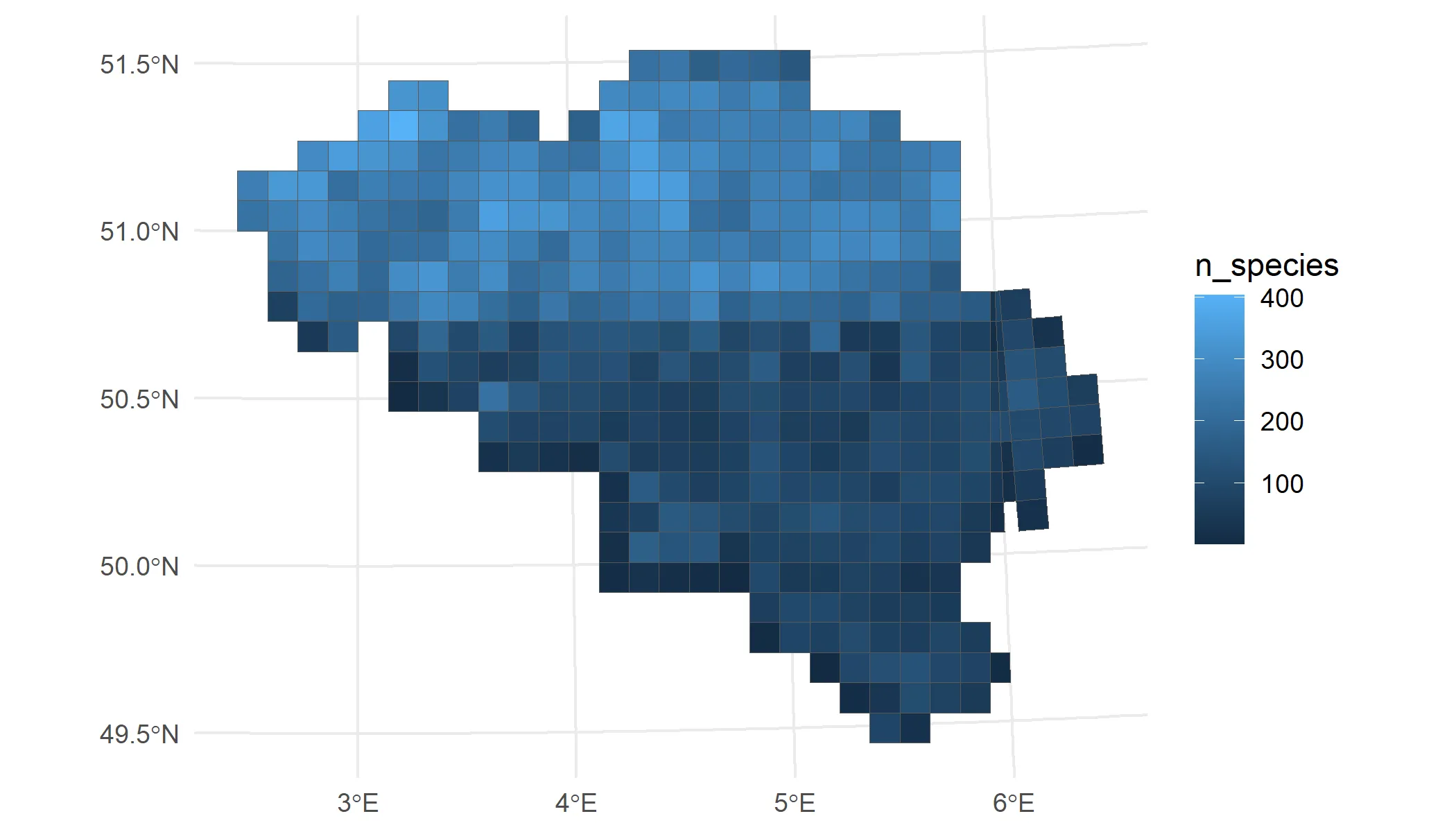
We now process the cleaned data cube using the b3gbi package (v0.4.0), which prepares the data for indicator calculations.
bird_cube_processed <- process_cube( bird_cube_belgium_clean, cols_occurrences = "n")bird_cube_processed#>#> Processed data cube for calculating biodiversity indicators#>#> Date Range: 2000 - 2024#> Single-resolution cube with cell size 10km ^2#> Number of cells: 379#> Grid reference system: mgrs#> Coordinate range:#> xmin xmax ymin ymax#> 2.428844 6.334746 49.445981 51.444030#>#> Total number of observations: 17609047#> Number of species represented: 733#> Number of families represented: 95#>#> Kingdoms represented: Data not present#>#> First 10 rows of data (use n = to show more):#>#> # A tibble: 557,608 × 11#> year cellCode taxonKey scientificName family obs minCoordinateUncerta…¹#> <dbl> <chr> <dbl> <chr> <chr> <dbl> <dbl>#> 1 2000 31UDS65 2473958 Perdix perdix Phasi… 1 3536#> 2 2000 31UDS65 2474156 Coturnix coturnix Phasi… 1 3536#> 3 2000 31UDS65 2474377 Fulica atra Ralli… 5 1000#> 4 2000 31UDS65 2475443 Merops apiaster Merop… 6 1000#> 5 2000 31UDS65 2480242 Vanellus vanellus Chara… 1 3536#> 6 2000 31UDS65 2480637 Accipiter nisus Accip… 1 3536#> 7 2000 31UDS65 2481172 Larus marinus Larid… 1 3536#> 8 2000 31UDS65 2481174 Larus fuscus Larid… 1 3536#> 9 2000 31UDS65 2481890 Phalacrocorax ca… Phala… 2 1000#> 10 2000 31UDS65 2482054 Podiceps cristat… Podic… 5 1000#> # ℹ 557,598 more rows#> # ℹ abbreviated name: ¹minCoordinateUncertaintyInMeters#> # ℹ 4 more variables: familyCount <dbl>, xcoord <dbl>, ycoord <dbl>,#> # resolution <chr>With the processed cube, we can reproduce a species richness map similar to the one created earlier.
bird_cube_richness_map <- obs_richness_map(bird_cube_processed)plot(bird_cube_richness_map)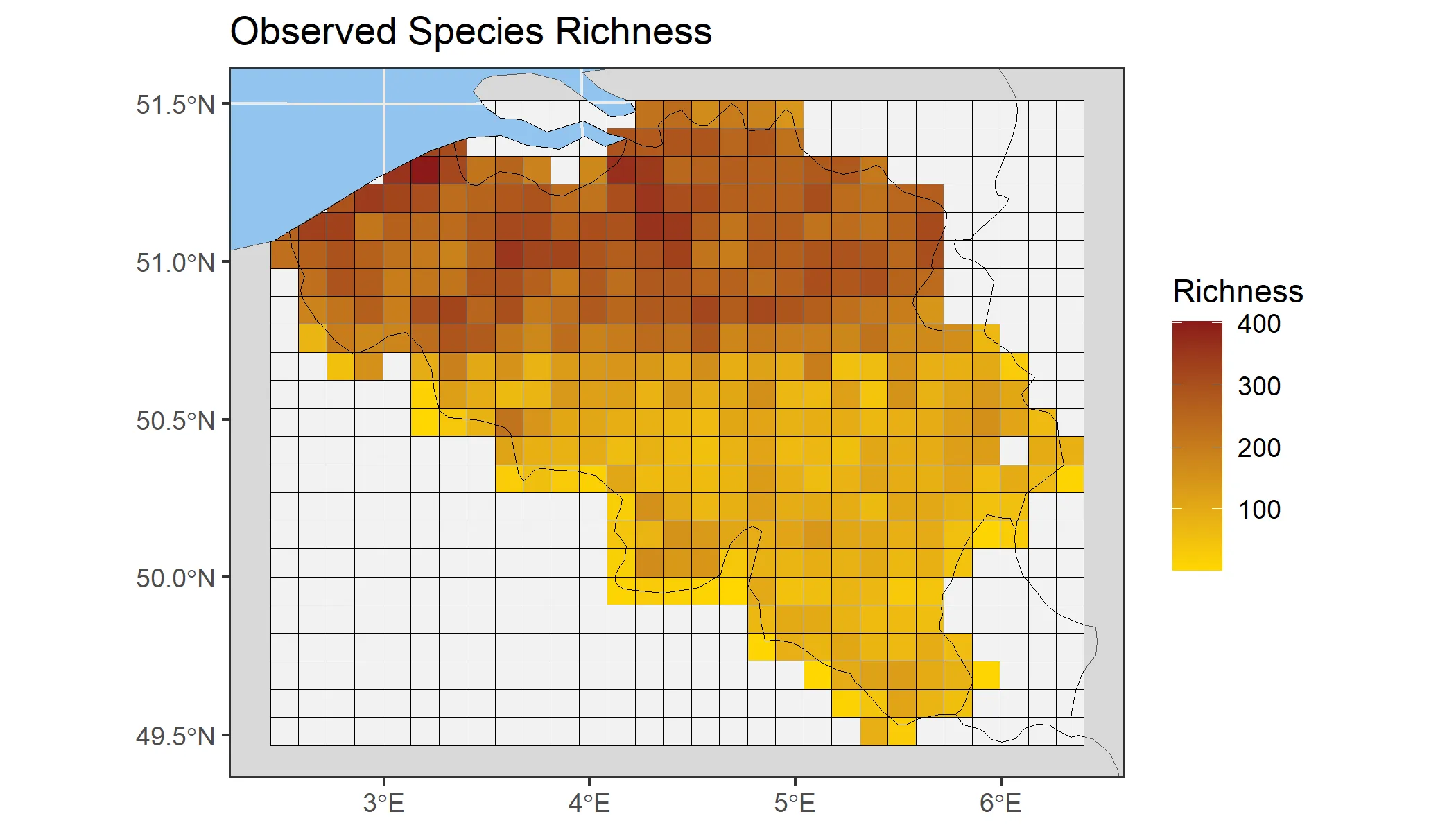
We can also calculate other biodiversity indicators. In the example below, we generate a time series of observed species richness. Confidence intervals are omitted here to reduce computation time.
bird_cube_richness_ts <- obs_richness_ts(bird_cube_processed, ci_type = "none")plot(bird_cube_richness_ts)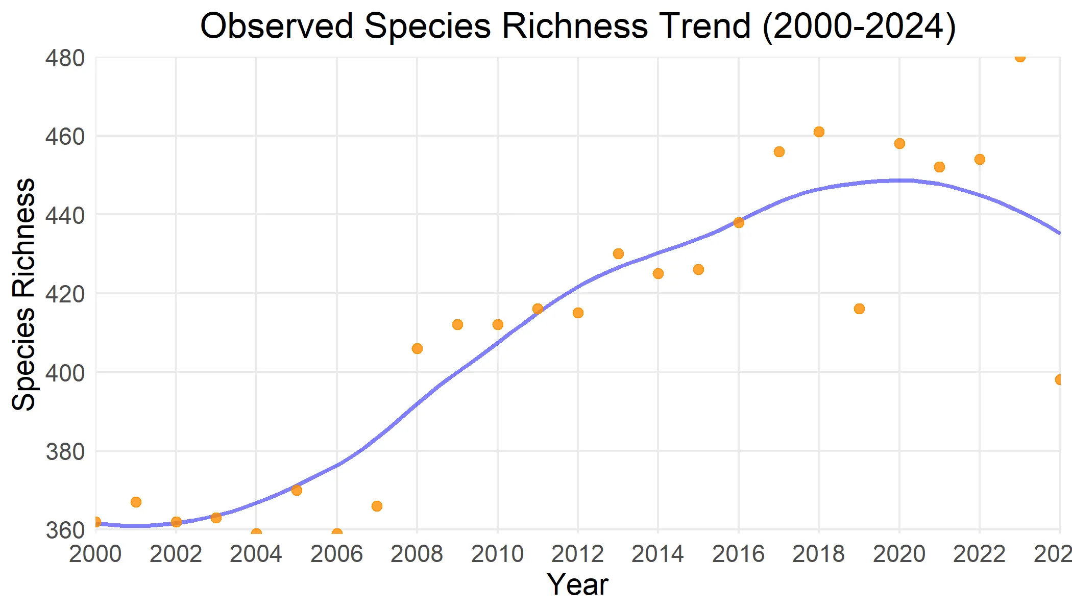
Note: The example demonstrates the use of the b3data resources, and is not intended as an example of rigorous ecological analysis. The spatial and temporal patterns shown in the outputs below primarily reflect the data coverage in GBIF, and may not reflect actual biodiversity patterns.
Contributing and reporting issues
How to contribute?
- Before contributing, check the “Contributing Guidelines” of the b3data-scripts repository.
- Fork the b3data-scripts repository.
- Follow the instructions in the README to set up the workflow.
- Submit a pull request for your changes.
- Submission of (a) resource(s) to the data package can also be requested in an issue in the repository and added by the maintainers of the data package itself.
Reporting bugs or suggesting improvements
- If you encounter a problem or like to suggest an improvement, open an issue in the b3data-scripts repository.
- Be as detailed as possible when describing the issue, including R session info, error messages, and reproducible examples if applicable.