Guide to Dissimilarity Cubes
This guide introduces Dissimilarity Cubes (DCs)—a reproducible, spatially explicit framework for analysing compositional turnover and community reorganisation using species occurrence data. The Dissimilarity Cube operates at the community level, mapping how assemblages differ across space, environment, and scenarios, and how these patterns may change under future conditions.
Rather than focusing on individual species, the Dissimilarity Cube characterises emergent biodiversity structure, enabling the identification of ecological regions, turnover regimes, and areas at risk of novel or unstable community configurations.
How to cite
Section titled “How to cite”If you use Dissimilarity Cubes in your work, please cite:
MacFadyen S, Cortès Lobos RB, Di Musciano M, Hui C, Rocchini D (2025). Documentation on modelled data cubes. B3 project deliverable D4.1.
Motivation and scope
Section titled “Motivation and scope”Understanding biodiversity change requires more than tracking species gains and losses. Ecological systems are structured by patterns of co-occurrence, shaped by environmental filtering, dispersal limitation, historical contingencies, and sampling processes. These forces operate across spatial scales, producing structured turnover in community composition.
Traditional β-diversity metrics typically quantify pairwise differences between sites, but they provide limited insight into how assemblages reorganise collectively across landscapes. The Dissimilarity Cube addresses this limitation by extending turnover analysis to multisite contexts, allowing biodiversity structure to be examined across scales, orders of species overlap, and environmental gradients.
The framework is particularly well suited to macroscale biodiversity monitoring, bioregionalisation, and scenario-based forecasting under climate or land-use change.
What is a Dissimilarity Cube?
Section titled “What is a Dissimilarity Cube?”A Dissimilarity Cube is a multi-dimensional data structure that organises compositional dissimilarity metrics across a harmonised spatial grid. Each grid cell represents a local assemblage, and dissimilarity is quantified among sets of cells using order-wise turnover metrics, most notably zeta (ζ) diversity.
The cube integrates:
- species occurrence data aggregated to a common spatial grain,
- environmental and spatial predictors,
- multisite dissimilarity measures,
- modelled relationships between turnover and environmental gradients.
By storing these components within a unified structure, the Dissimilarity Cube enables consistent slicing across space, predictors, dissimilarity orders, and scenarios, supporting both exploratory and inferential analyses of biodiversity turnover.
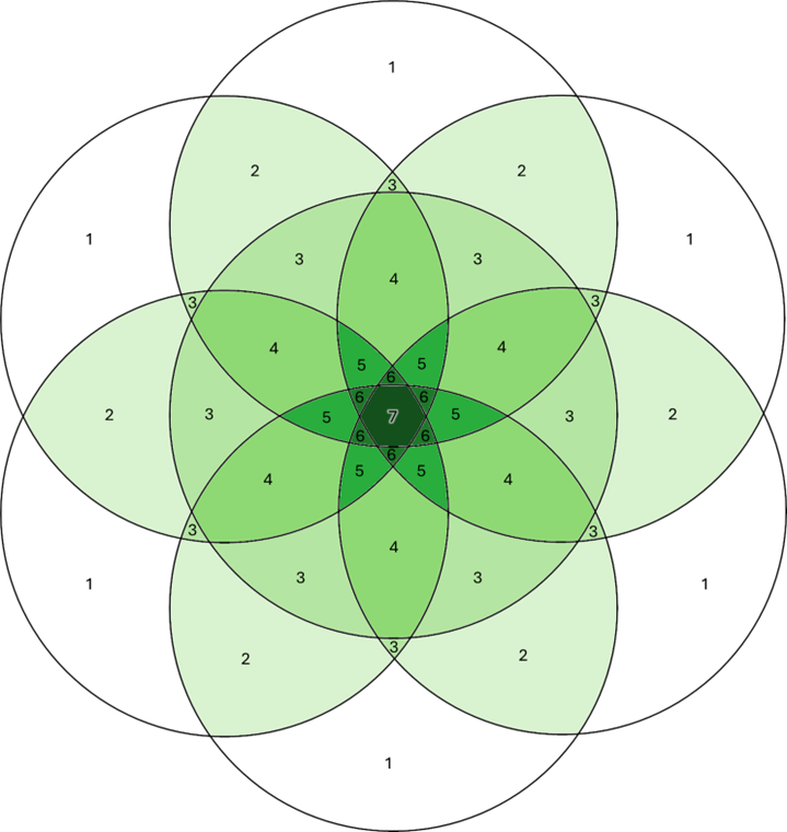
Figure 1. Conceptual illustration of zeta (ζ) diversity across multiple sites.
Ecological foundations
Section titled “Ecological foundations”Compositional turnover beyond pairwise β-diversity
Section titled “Compositional turnover beyond pairwise β-diversity”Compositional turnover reflects how species assemblages change across space and environment. While pairwise β-diversity captures local differences between sites, it cannot represent how groups of sites share or lose species collectively. This limits inference about regional structure, persistence of widespread taxa, and the processes shaping biodiversity across scales.
The Dissimilarity Cube formalises turnover in a multisite framework, enabling detection of compositional regimes, ecological stability, and scale-dependent drivers of biodiversity change.
Zeta diversity and order-wise turnover
Section titled “Zeta diversity and order-wise turnover”Zeta diversity (ζ-diversity) generalises β-diversity by measuring the number of species shared among i sites. Low orders (e.g. ζ₂) emphasise rare and localised species and approximate conventional β-diversity, while higher orders capture overlap among many sites and therefore reflect widespread, persistent taxa.
The decline of ζ with increasing order provides a continuous description of turnover across spatial scales, linking α-, β-, and γ-diversity within a single analytical framework. Crucially, different ζ-orders capture different ecological processes, rather than simply rescaling pairwise turnover.
Linking turnover to environment: ζ-MS-GDM
Section titled “Linking turnover to environment: ζ-MS-GDM”To relate multisite turnover to environmental gradients, the Dissimilarity Cube uses Multi-Site Generalised Dissimilarity Modelling (ζ-MS-GDM). This approach models order-wise dissimilarity as a function of environmental and spatial predictors using i-spline transformations, allowing non-linear, threshold-like responses.
ζ-MS-GDM produces:
- partial-dependence curves describing how predictors erode shared species pools,
- variance partitioning between environmental and spatial drivers,
- order-specific insights into the mechanisms shaping biodiversity structure.
Workflow overview
Section titled “Workflow overview”The Dissimilarity Cube workflow integrates biodiversity data, environmental predictors, and multisite turnover metrics into a fully reproducible pipeline implemented through the dissmapr framework.
Data acquisition and aggregation
Section titled “Data acquisition and aggregation”Species occurrence records are compiled and aggregated to a regular spatial grid, defining local assemblages. Environmental predictors, such as climate and sampling-effort layers, are extracted and aligned to the same grid. This harmonisation ensures that compositional and environmental data are directly comparable.
Data screening and preparation
Section titled “Data screening and preparation”Prior to analysis, data are screened for sampling bias, collinearity among predictors, and inconsistencies in spatial coverage. Effort diagnostics are explicitly incorporated to distinguish ecological signals from artefacts of observation intensity.
Computation of order-wise dissimilarity
Section titled “Computation of order-wise dissimilarity”ζ-diversity is computed across a range of orders (ζ₂–ζₙ), producing dissimilarity matrices that describe turnover from pairwise to multisite contexts. These metrics form the core informational content of the Dissimilarity Cube.
Modelling and prediction
Section titled “Modelling and prediction”ζ-MS-GDM models are fitted to link turnover to environmental and spatial gradients. Fitted models are then used to predict continuous turnover surfaces across the study region and, where applicable, under future environmental scenarios.
Spatial synthesis and scenario analysis
Section titled “Spatial synthesis and scenario analysis”Predicted turnover surfaces can be clustered into bioregions, representing spatially coherent units of community composition. The same workflow can be applied to future scenarios, enabling comparison of present and projected compositional structure and identification of regions prone to reorganisation.
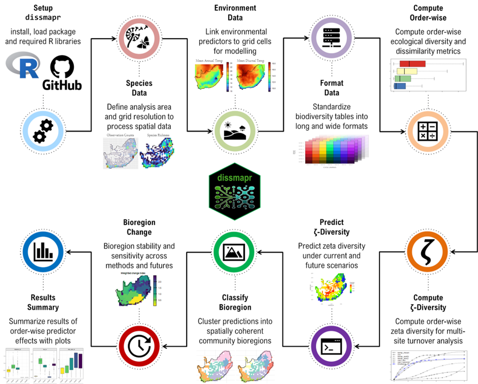
Figure 2. Conceptual workflow of the Dissimilarity Cube implemented in dissmapr.
Technical implementation
Section titled “Technical implementation”The Dissimilarity Cube is implemented in R using open-source packages, including dissmapr, zetadiv, terra, sf, and ggplot2. Each analytical step—from data harmonisation to modelling and mapping—is encapsulated in documented, parameterised functions.
This modular design ensures transparency, reproducibility, and flexibility across taxa, regions, spatial grains, and scenario sets.
Outputs and products
Section titled “Outputs and products”A Dissimilarity Cube produces a suite of complementary outputs, including:
- order-wise dissimilarity matrices (ζ₂–ζₙ),
- continuous spatial predictions of turnover,
- bioregional maps derived from clustering turnover surfaces,
- partial-dependence plots from ζ-MS-GDM,
- change and sensitivity maps comparing scenarios.
Together, these products describe how biodiversity composition varies across space, scale, and environmental change.
Applications
Section titled “Applications”Dissimilarity Cubes support a wide range of biodiversity analyses, including:
- monitoring compositional change across spatial scales,
- detecting ecological thresholds and transition zones,
- objective bioregionalisation for conservation planning,
- forecasting community reorganisation under future scenarios,
- sensitivity analysis to modelling and clustering choices.
Worked example: Lepidoptera in South Africa
Section titled “Worked example: Lepidoptera in South Africa”A large-scale application analyses butterfly assemblages in South Africa using over 55,000 occurrence records aggregated to a 0.5° grid. Occurrences are linked to climate predictors and sampling-effort layers, and ζ-diversity is computed across multiple orders.
ζ-MS-GDM results reveal a strong, order-dependent hierarchy in the drivers of turnover. At low orders (ζ₂), geographic distance dominates, reflecting local distance decay. At intermediate orders (ζ₃–ζ₄), climatic heterogeneity becomes increasingly influential. At high orders (ζ₅–ζ₆), turnover is governed primarily by climatic envelopes and sampling completeness, indicating processes controlling regional persistence of widespread species.
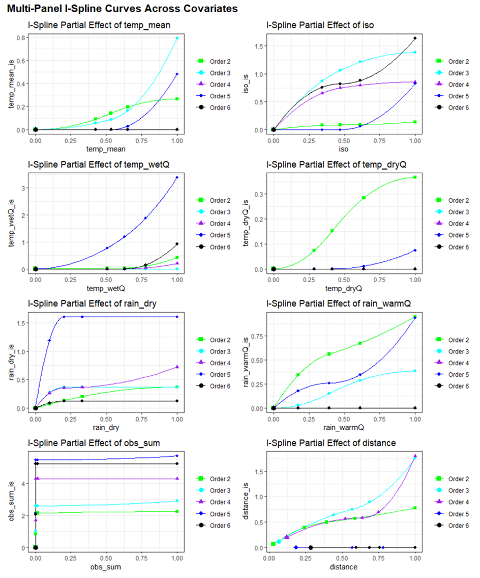
Figure 3. Partial-dependence curves for environmental predictors across ζ-orders.
Interpreting i-spline responses
Section titled “Interpreting i-spline responses”The geometry of i-spline curves provides direct ecological insight. Spline height reflects the relative importance of a predictor in eroding shared species pools, while steep early rises indicate thresholds where small environmental changes produce rapid turnover. Flattening tails suggest saturation effects, and distance splines quantify residual spatial decay after accounting for environmental structure.
Collectively, these patterns reveal which gradients matter most, and at which spatial scale.
Spatial prediction and bioregionalisation
Section titled “Spatial prediction and bioregionalisation”Spatial predictions of ζ₂ produce smooth turnover gradients across South Africa, highlighting regions of strong environmental contrast or isolation. Clustering these surfaces yields coherent bioregions that are largely consistent across algorithms, with local boundary uncertainty aligning with ecological transition zones.
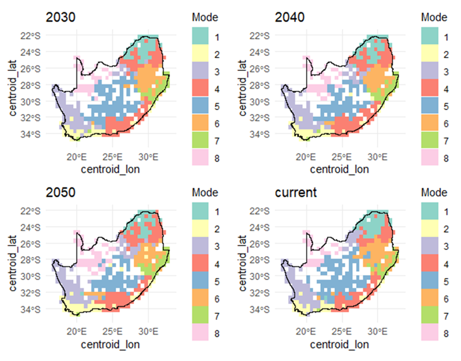
Figure 4. Bioregional configurations under current and future scenarios.
Sensitivity and robustness
Section titled “Sensitivity and robustness”Sensitivity analyses explicitly separate methodological uncertainty from environmental change signals. Regions stable across clustering methods but sensitive to climate projections indicate robust ecological reorganisation, whereas areas sensitive to both require cautious interpretation.
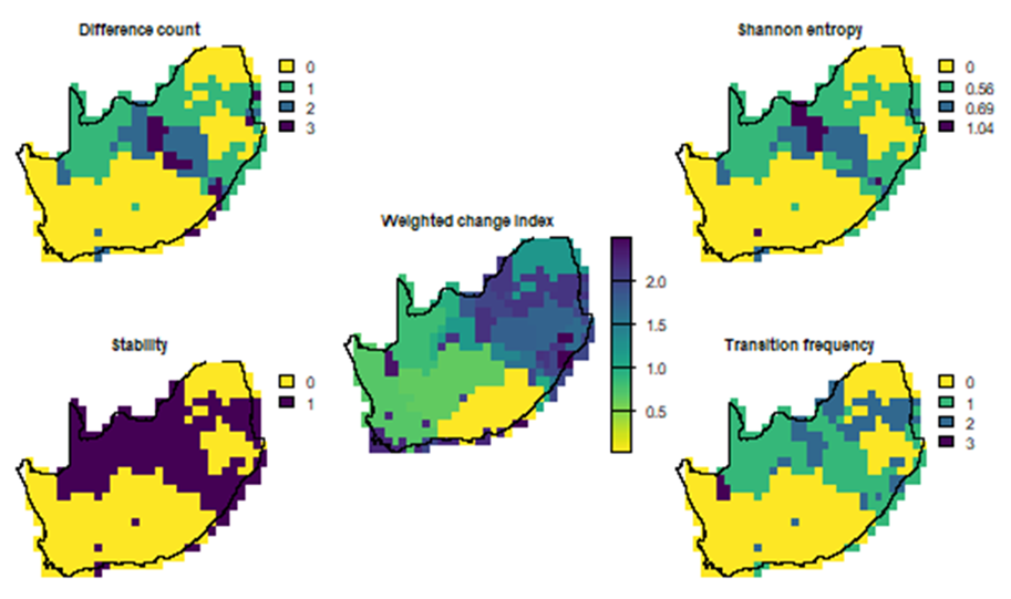
Figure 5. Sensitivity of bioregional delineation to clustering method.
Reproducibility and quality assurance
Section titled “Reproducibility and quality assurance”All analyses are fully scripted and version-controlled, with explicit handling of spatial reference systems, effort diagnostics, predictor screening, and parameterisation. Each output can be traced back to raw inputs, ensuring auditability and scientific robustness.
Synthesis and future directions
Section titled “Synthesis and future directions”The Dissimilarity Cube provides a scale-explicit framework for analysing biodiversity turnover beyond pairwise comparisons. By integrating ζ-diversity, spatial modelling, and scenario analysis, it reveals order-dependent ecological processes and supports robust assessment of compositional change under global change.
Future developments should prioritise improved bias correction, integration of land-use and dispersal constraints, and systematic comparisons across taxa, regions, and spatial grains.