Guide to Invasibility Cubes
This guide introduces Invasibility Cubes—a transparent, reproducible framework for quantifying invasion fitness, species invasiveness, and site invasibility by integrating species occurrences, Invasive Alien Species (IAS) lists, functional traits, and community interaction structure. The Invasibility Cube is designed for applications where invasion risk cannot be inferred from abiotic suitability alone, because establishment depends on the joint action of trait–environment matching, trait-mediated competition, and resident community saturation.
Implemented in the invasimapr R package, the cube organises invasion processes into a consistent multidimensional structure that resolves invasion outcomes at the site × invader level. This enables direct comparison of invasion risk across landscapes, taxa, and scenarios, and supports decision-ready outputs for horizon scanning, surveillance prioritisation, and ecosystem management.
How to cite
Section titled “How to cite”If you use Invasibility Cubes in your work, please cite:
MacFadyen S, Trekels M, Yahaya M, Landi P, Hui C (2024). Specification for invasibility cubes and their production. https://docs.b-cubed.eu/guides/invasibility-cube/
Motivation and scope
Section titled “Motivation and scope”Biological invasions are a major driver of biodiversity loss and ecosystem change, yet invasion outcomes remain difficult to predict because establishment success is rarely controlled by a single driver. Many risk maps emphasise abiotic suitability, but invaders also face strong constraints from resident communities through competition and niche overlap. Conversely, apparently “resistant” communities can become vulnerable when invaders occupy underfilled trait space or when environmental change shifts the balance of abiotic opportunity and biotic resistance.
The Invasibility Cube addresses this complexity by embedding invasion ecology into a shared analytical geometry that integrates three ingredients: (i) invader traits, (ii) environmental conditions, and (iii) resident community structure. The result is a mechanistic, spatially explicit view of invasion potential: not only where invaders could persist, but also where they can establish given trait overlap and competitive loading.
What is an Invasibility Cube?
Section titled “What is an Invasibility Cube?”An Invasibility Cube is a multi-dimensional data structure that estimates invasion fitness for a set of candidate invaders across a set of sites, given local environments and resident communities. The cube is built from three interoperable data blocks:
- an environment tensor describing sites across environmental variables (and optionally scenarios),
- a community tensor describing resident assemblages at sites (and optionally scenarios),
- a trait matrix describing invader and resident species in a shared functional trait space.
These inputs support a workflow that (a) constructs a shared trait geometry, (b) estimates site-level predictors of abiotic opportunity and biotic resistance, and (c) synthesises these components into a site × invader invasion-fitness surface. From this surface, two headline indicators are derived: species invasiveness (who tends to establish) and site invasibility (where invasions are most likely), along with trait-level diagnostics to explain why.
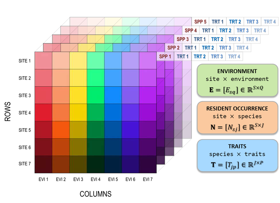
Figure 1. Interoperable environment, community, and trait structures underpinning the Invasibility Cube.
Core concepts
Section titled “Core concepts”Trait-centred invasion ecology in a shared geometry
Section titled “Trait-centred invasion ecology in a shared geometry”The Invasibility Cube formalises the principle that establishment success depends jointly on abiotic suitability, biotic resistance, and invader traits. Rather than treating these as separate modelling steps, the cube embeds them in a shared trait–environment representation. Resident communities define the set of trait strategies currently supported at each site, while candidate invaders are positioned relative to this resident “trait cloud”. This geometric framing provides an interpretable bridge between measurable traits and invasion outcomes.
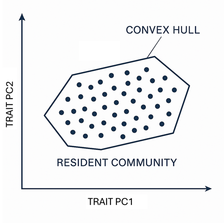
Figure 2. Conceptual trait-space geometry: residents form a trait cloud; invaders succeed or fail depending on trait novelty/overlap and site context.
Shared trait–environment space and biotic resistance geometry
Section titled “Shared trait–environment space and biotic resistance geometry”The shared trait–environment space is the cube’s conceptual core. Communities are represented not only by species counts, but by the distribution of functional strategies they contain. In this space, strong niche overlap between invader traits and resident traits implies higher expected competitive pressure, whereas trait novelty can reduce direct overlap and potentially increase establishment—provided the invader is also compatible with local environmental conditions.
This framing clarifies an important point: richness alone is an unreliable proxy for resistance. A community can be species-rich but functionally underfilled (low saturation), or species-poor but tightly packed in trait space (high overlap and competition). The cube therefore distinguishes how many species occur from how strongly they constrain invaders.
Invasion fitness (λ)
Section titled “Invasion fitness (λ)”Invasion fitness (λᵢₛ) represents the per-capita growth rate of a rare invader i at site s, conditional on local environment and resident community structure. In practice, λᵢₛ is decomposed into interpretable components that capture distinct processes:
- Abiotic suitability: how well invader traits align with the site’s environment (opportunity for growth),
- Trait-mediated crowding: competitive penalty arising from functional overlap with residents,
- Site saturation: cumulative competitive loading reflecting community “filledness”.
When λᵢₛ > 0, abiotic gains outweigh biotic penalties and establishment is expected; when λᵢₛ < 0, invaders are excluded. Fitness values are typically transformed into establishment probabilities using logistic/probit links or threshold rules, yielding a decision-ready site × invader likelihood surface.
Derived indicators: invasiveness and invasibility
Section titled “Derived indicators: invasiveness and invasibility”The invasion-fitness surface can be summarised in two complementary ways. Species invasiveness measures the propensity of invader i to establish across sites (e.g., the proportion of sites with high establishment probability), while site invasibility measures the openness of site s to invasion (e.g., the expected number or proportion of invaders that can establish). Trait-level summaries quantify which traits contribute most to establishment success, supporting interpretable screening and mechanistic explanation.
Workflow overview
Section titled “Workflow overview”The Invasibility Cube workflow progresses from harmonised ecological inputs to invasion fitness estimation and decision-ready summaries. Although implementations vary by dataset, the core stages are consistent.
Data assembly and harmonisation
Section titled “Data assembly and harmonisation”The workflow begins with the construction of aligned site-level structures describing environment, resident community composition, and species traits. This alignment step is not merely technical: invasion outputs are only meaningful if traits, occurrences, and environments refer to the same entities and spatial units. The pipeline therefore standardises taxonomies, resolves spatial geometry, and enforces consistent trait schemas across residents and invaders (real or simulated).
Trait compilation and interpretability scaffolding
Section titled “Trait compilation and interpretability scaffolding”Trait datasets are frequently incomplete, uneven across taxa, or inconsistent across sources. The workflow addresses this by harmonising a species-by-traits table and attaching interpretability scaffolding (e.g., taxonomy, metadata) so that later invasion predictions can be traced back to functional axes rather than remaining opaque statistical outputs. This step is crucial when the goal is to translate results into screening rules or management-relevant narratives.
Trait space construction and crowding metrics
Section titled “Trait space construction and crowding metrics”A reduced trait space is constructed (commonly via PCoA on Gower distances), and resident communities are represented as trait distributions within this space. Diagnostics quantify trait density structure, resident niche envelopes (e.g., convex hulls), and invader centrality/novelty (e.g., Mahalanobis distance). From these, site-weighted crowding measures are derived to represent trait-mediated biotic resistance.
This is typically the first step where the cube becomes mechanistic: invasion potential is interpreted through an invader’s position relative to resident strategies, rather than only through environmental correlations.
Resident predictors: separating opportunity from resistance
Section titled “Resident predictors: separating opportunity from resistance”The cube then estimates resident-derived predictors that parameterise invasion fitness. These predictors distinguish abiotic opportunity from multiple forms of biotic resistance, commonly including:
- a resident-calibrated abiotic suitability layer,
- a trait-similarity crowding layer describing overlap-based competition,
- a site saturation layer capturing community filledness/competitive loading.
These layers are explicitly designed to decouple resistance from richness, revealing where communities are competitively packed versus merely species-rich, and where abiotic opportunity is high but resistance may still prevent establishment.
Sensitivities and invader prediction on resident scales
Section titled “Sensitivities and invader prediction on resident scales”Invasion processes are rarely uniform across trait strategies. The workflow therefore estimates trait- (and optionally site-) varying sensitivities that modulate how abiotic and biotic predictors translate into invasion fitness. Invader predictors are then projected onto resident-standardised scales to prevent scale leakage and to ensure comparability between residents and candidate invaders.
Invasion fitness and establishment probability
Section titled “Invasion fitness and establishment probability”Finally, the model synthesises opportunity and resistance into invasion fitness (λ) and transforms λ into establishment probability (P). This yields the central product of the cube: a site × invader surface that answers, directly and explicitly, which invaders can establish where, given both environmental conditions and resident community constraints.
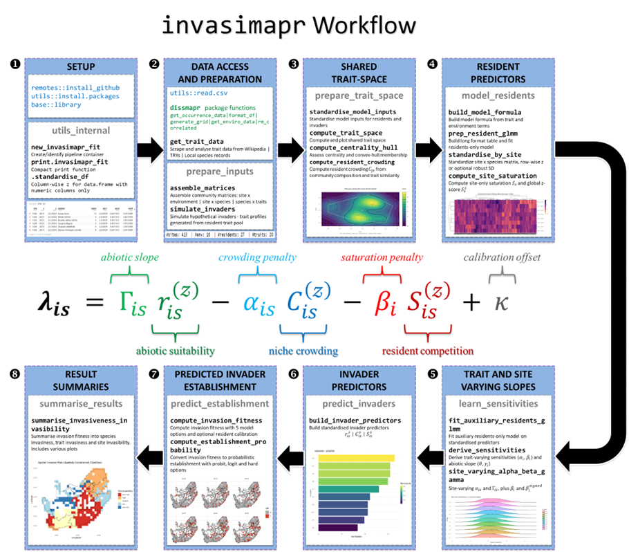
Figure 3. Conceptual workflow linking data preparation, trait-space modelling, resident predictors, and invasion fitness estimation.
Technical implementation
Section titled “Technical implementation”Invasibility Cubes are implemented in R via invasimapr, using modular wrapper functions corresponding to the conceptual steps of the workflow. A typical pipeline includes:
prepare_inputs()to align sites, environments, communities, and traits,prepare_trait_space()to construct trait geometry and crowding indices,model_residents()to estimate resident predictors such as saturation and baseline suitability,learn_sensitivities()to capture trait- and site-varying effects,predict_invaders()to generate invader predictors on resident-calibrated scales,predict_establishment()to compute invasion fitness and establishment probabilities,summarise_results()to derive site-, species-, and trait-level indicators.
This structure ensures conceptual assumptions map directly to code, supporting reproducible scientific analysis and policy-relevant deployment.
Outputs and products
Section titled “Outputs and products”The Invasibility Cube produces a family of linked outputs that describe invasion risk at multiple ecological levels. Core outputs include invasion-fitness surfaces (λ) and establishment probabilities (P) across sites and candidate invaders, alongside summary rankings of species invasiveness and spatial maps of site invasibility. Trait-effect summaries and diagnostic plots provide mechanistic interpretation, allowing invasion risk to be explained in terms of functional strategies and the balance of abiotic opportunity versus biotic resistance.
Applications
Section titled “Applications”Invasibility Cubes support invasion risk assessment and horizon scanning by identifying high-risk invaders and invasion-prone regions. They can be used to prioritise surveillance and early detection, evaluate trait-based screening rules, explore how invasibility changes under environmental scenarios, and communicate mechanistic explanations of why certain communities or regions are more vulnerable. Because outputs are resolved at the site × invader level, the cube naturally supports targeted, region-specific management rather than uniform, one-size-fits-all strategies.
Worked example: Lepidoptera in South Africa
Section titled “Worked example: Lepidoptera in South Africa”A demonstrative application analyses Afrotropical Lepidoptera across South Africa using gridded occurrence data, climatic predictors, and functional traits. The workflow begins by harmonising site, environment, and community matrices and compiling a trait dataset aligned between residents and candidate invaders. A shared trait space is then constructed to quantify invader novelty and resident crowding, after which resident predictors are fitted to separate abiotic opportunity from biotic resistance mechanisms.
Results show that invasion success is strongly spatially heterogeneous and emerges from trade-offs between abiotic suitability, trait overlap, and saturation. Regions with high abiotic opportunity but weak crowding and low saturation exhibit elevated invasibility, whereas sites with strong functional overlap and high competitive loading remain resistant even under favourable environments.
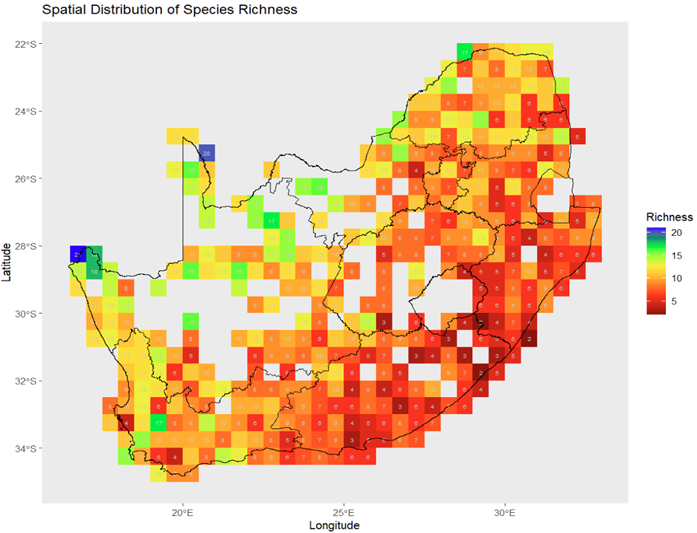
Figure 4. Resident richness provides baseline context, but resistance emerges mechanistically through trait overlap and saturation rather than richness alone.
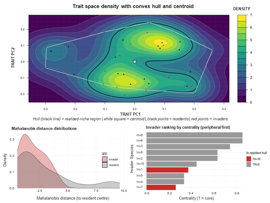
Figure 5. Trait-space diagnostics: resident density structure, niche envelopes, and invader novelty/centrality.
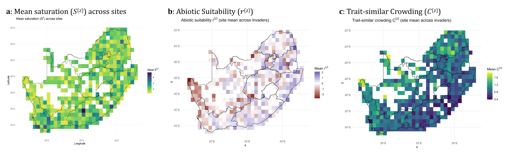
Figure 6. Resident predictors separating abiotic opportunity from biotic resistance mechanisms.
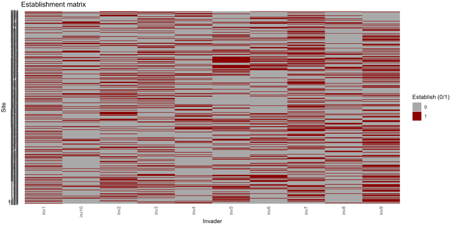
Figure 7. Site × invader establishment outcomes reveal structured, heterogeneous invasion risk.
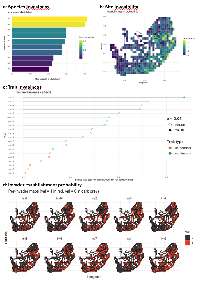
Figure 8. Decision-ready summaries: species invasiveness, site invasibility, and trait drivers of establishment.
Reproducibility and quality assurance
Section titled “Reproducibility and quality assurance”Quality assurance is enforced through standardised data schemas, explicit spatial alignment, transparent trait and environmental scaling, and modular parameterisation of each modelling stage. Intermediate objects are preserved to support auditing and sensitivity checks, and implementations are designed for version control and reproducibility from raw inputs through to final invasion indicators.
Synthesis and future directions
Section titled “Synthesis and future directions”The Invasibility Cube operationalises a trait-centred, community-aware approach to invasion risk assessment by explicitly integrating abiotic suitability, trait-mediated competition, and community saturation within a single analytical structure. This enables invasion outcomes to be interpreted mechanistically and mapped consistently across landscapes.
Future developments should prioritise temporal dynamics, propagule pressure, alternative similarity kernels for crowding, explicit detection and sampling models, and scenario propagation under climate and land-use change. Repeated analyses through time will strengthen the cube’s role as a monitoring and decision-support tool for biodiversity management under global change.