Specification for suitability cubes and their production
This guide introduces Suitability Cubes (SCs)—a standardized, reproducible data cube developed within WP4 of the B3 project to support habitat suitability modelling and the critical evaluation of Species Distribution Models (SDMs). The Suitability Cube is designed as an evaluation layer that complements SDM outputs by making explicit where predictions are environmentally supported and where they rely on extrapolation.
Rather than proposing a new modelling algorithm, the Suitability Cube provides a structured way to align model predictions with diagnostics of environmental representativeness across space, time, and taxa. This enables more transparent interpretation of SDM results, particularly under climate change scenarios.
How to cite
Section titled “How to cite”If you use Suitability Cubes in your work, please cite:
MacFadyen S, Cortès Lobos RB, Di Musciano M, Hui C, Rocchini D (2025). Documentation on modelled data cubes. B3 project deliverable D4.1.
This guide builds on methodological developments described in:
Cortès Lobos RB, Di Musciano M, Martini M, Rocchini D (2024). M11: Code development for predictive habitat suitability modelling.
Cortès Lobos RB, Di Musciano M, Rocchini D (2025). M12: Code testing for predictive habitat suitability modelling.
Motivation and scope
Section titled “Motivation and scope”Species Distribution Models are widely used to infer habitat suitability across geographic space and to project potential shifts under future environmental conditions. However, SDM outputs are often interpreted without explicitly accounting for the degree to which projected environments are represented in the data used to train the models. As a result, predictions may appear precise even when they rely heavily on environmental extrapolation.
The Suitability Cube addresses this limitation by embedding indicators of environmental novelty, niche breadth, and model applicability directly alongside SDM outputs. This allows users to distinguish between areas where predictions are environmentally well supported and areas where model transferability is uncertain. In doing so, the Suitability Cube supports more cautious, transparent, and defensible use of SDMs in biodiversity assessment and decision-making.
What is a Suitability Cube?
Section titled “What is a Suitability Cube?”A Suitability Cube is a multi-dimensional data structure that organises SDM-related diagnostics across three core dimensions: space, taxa, and time. Spatially, the cube is defined over a regular grid of cells; taxonomically, it spans one or more species; temporally, it includes present-day conditions and one or more future scenarios or time periods.
Within this shared structure, the cube stores multiple indicators that describe how model predictions relate to the environmental conditions used for calibration. By aligning all indicators on the same grid and dimensions, the Suitability Cube enables direct comparison across species, locations, and scenarios, while maintaining full consistency among inputs.
Importantly, the Suitability Cube does not replace SDMs. Instead, it complements them by answering a different question: where are SDM predictions environmentally supported, and where should they be treated with caution?
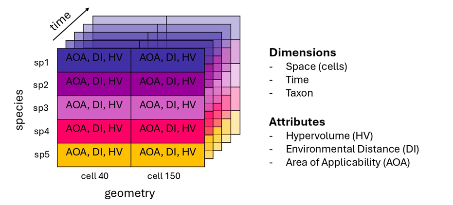
Figure 1. Conceptual structure of the Suitability Cube, organised along spatial, taxonomic, and temporal dimensions.
Core indicators
Section titled “Core indicators”The informational content of the Suitability Cube is defined by three complementary indicators: Hypervolume (HV), Environmental Distance (DI), and Area of Applicability (AOA). Together, these indicators characterise niche breadth, environmental novelty, and model validity.
Hypervolume (HV)
Section titled “Hypervolume (HV)”The Hypervolume represents a species’ realised environmental niche as an n-dimensional region of predictor space, following Hutchinson’s niche concept. Each dimension corresponds to a standardised environmental variable, such as temperature or precipitation. Hypervolumes are estimated from observed species occurrences using Gaussian kernel density estimation and are computed for present-day conditions only.
HV provides a quantitative summary of sampled niche breadth. Larger hypervolumes indicate that a species occupies a wider range of environmental conditions in the available data, although interpretation must consider sampling density and potential bias in occurrence records.
Environmental Distance (DI)
Section titled “Environmental Distance (DI)”The Environmental Distance, or Dissimilarity Index (DI), measures how different the environmental conditions at a given location are from those represented in the training data. DI is computed in a standardised, importance-weighted predictor space and is normalised using the empirical distribution of distances among training samples.
Low DI values indicate environments that are well represented in the calibration data, whereas high DI values signal increasing novelty and potential extrapolation. Because DI is computed for both present and future conditions, it provides a consistent basis for evaluating model transferability through time.
Area of Applicability (AOA)
Section titled “Area of Applicability (AOA)”The Area of Applicability (AOA) defines the spatial domain within which SDM predictions are considered environmentally valid. AOA is derived by thresholding DI based on the empirical distribution of distances among training samples. Locations exceeding this threshold are classified as lying outside the model’s applicable environmental domain.
AOA therefore provides a binary mask that separates environmentally supported predictions from those that should be interpreted with caution.
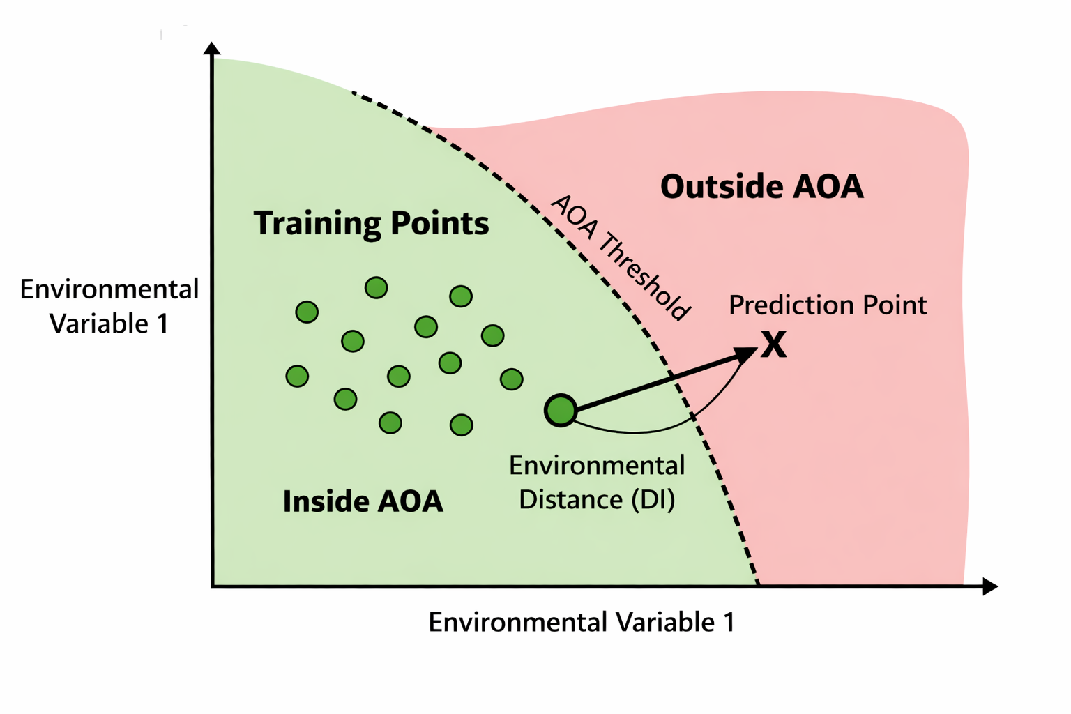
Figure 2. Conceptual relationship between Environmental Distance (DI) and Area of Applicability (AOA).
Workflow overview
Section titled “Workflow overview”Producing a Suitability Cube involves four main stages: data acquisition, pre-processing, indicator computation, and cube construction. Each stage is designed to ensure consistency between SDM inputs and evaluation metrics.
Data acquisition
Section titled “Data acquisition”The workflow begins with the collection of species occurrence records (e.g. from GBIF) and environmental predictors for both present-day conditions and future scenarios. Predictors are typically drawn from climate datasets such as WorldClim or CMIP6. To reduce redundancy and multicollinearity, correlation-based variable selection is applied to the present-day predictors and carried forward consistently to future scenarios.
Pre-processing
Section titled “Pre-processing”All inputs are harmonised prior to analysis. Occurrence records are cleaned, deduplicated, and spatially filtered, while environmental rasters are aligned, cropped, and resampled to a common grid. Predictors are standardised using statistics derived from present-day conditions, ensuring comparability across time periods.
This harmonisation step ensures that SDMs and Suitability Cube indicators are derived from identical environmental representations.
Indicator computation
Section titled “Indicator computation”Using the processed inputs, hypervolumes are estimated for each species under present conditions. Environmental Distance is then computed for both present and future environments, and Area of Applicability is derived by thresholding DI. All indicators are calculated using the same predictors and occurrence data employed in SDM calibration.
Cube construction
Section titled “Cube construction”Indicators are aggregated onto the spatial grid and combined into a single multi-attribute cube with dimensions cell × taxon × time. Hypervolume values are stored as species-level attributes, while DI and AOA vary across space and time. The resulting cube provides a unified object for joint analysis and visualisation.
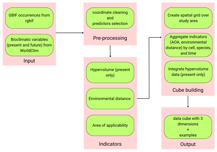
Figure 3. Overview of the Suitability Cube workflow.
Technical implementation
Section titled “Technical implementation”Suitability Cubes are implemented in R using modular, reproducible workflows. All settings are defined in a single user-controlled parameter list specifying species, spatial extent, resolution, climate scenarios, and modelling options. Helper functions handle data retrieval, alignment, variable selection, and indicator computation, while multi-dimensional cube objects are constructed using the stars package.
This design promotes transparency, reproducibility, and portability across regions, taxa, and modelling experiments.
Output structure
Section titled “Output structure”The final product is a multi-attribute environmental data cube containing continuous DI values, binary AOA masks, and species-level hypervolume estimates. Because all indicators share the same spatial, taxonomic, and temporal dimensions, the cube supports robust querying, comparison, and visualisation without additional alignment steps.
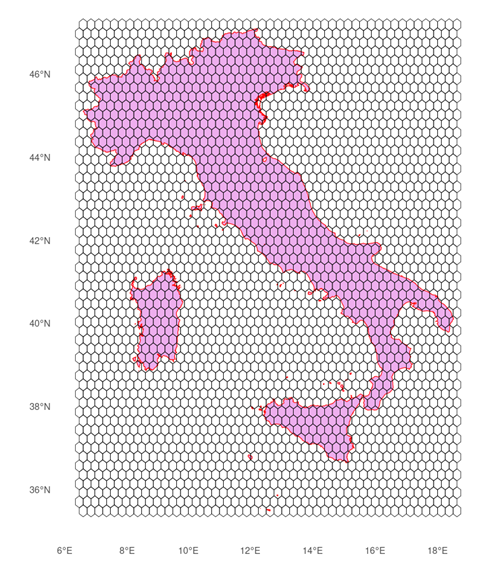
Figure 4. Dimensions and attributes of the Suitability Cube.
Applications
Section titled “Applications”Suitability Cubes can be used to identify environmentally unsupported SDM projections, compare exposure to novel conditions across species, constrain spatial prioritisation to areas of model validity, and communicate model limitations alongside predicted suitability patterns. By explicitly linking predictions to their environmental support, the Suitability Cube enhances both interpretability and scientific defensibility.
Worked example: amphibians in Italy
Section titled “Worked example: amphibians in Italy”A demonstrative application considers three amphibian species (Bufo bufo, Bufotes viridis, Bombina variegata) in Italy. After compiling present and future climate predictors and cleaning GBIF occurrence records, hypervolumes, environmental distance, and areas of applicability are computed and assembled into a Suitability Cube.
Results reveal increasing environmental novelty and contracting Areas of Applicability under future climate scenarios, indicating declining model transferability despite continued model predictions.
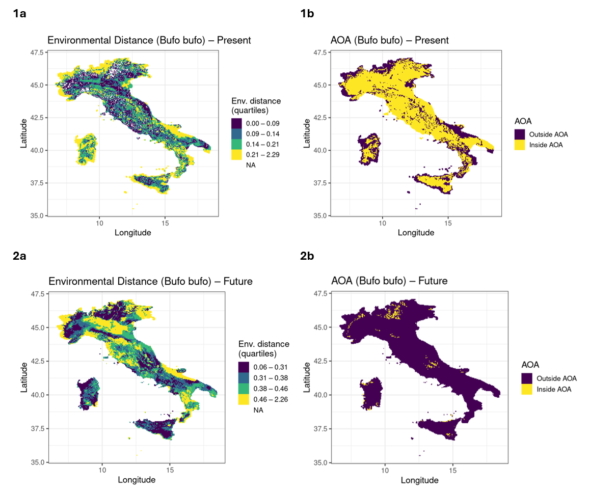
Figure 5. Environmental Distance and Area of Applicability for amphibians in Italy.
Reproducibility and future directions
Section titled “Reproducibility and future directions”The Suitability Cube workflow is fully scripted, version-controlled, and based on open-source tools. All indicators are traceable back to raw inputs, supporting auditability and quality assurance. Future extensions may incorporate land-use predictors, additional temporal horizons, broader taxonomic coverage, and systematic comparisons across SDM algorithms and spatial resolutions.
By embedding environmental applicability directly into SDM evaluation, Suitability Cubes provide a robust foundation for transparent biodiversity modelling under global change.