Calculating bootstrap confidence intervals

Introduction

When working with data cubes, it’s essential to understand the uncertainty surrounding derived statistics. This tutorial introduces the calculate_bootstrap_ci() function from dubicube, which uses bootstrap replications to estimate the confidence intervals around statistics calculated from data cubes.

Calculating bootstrap confidence intervals

In the bootstrap tutorial, we introduced bootstrapping as a way to assess the variability of statistics calculated from data cubes. Bootstrapping involves repeatedly resampling the dataset and recalculating the statistic to create a distribution of possible outcomes (= bootstrap replicates).

This tutorial builds on that foundation by showing how to compute confidence intervals from those bootstrap replicates. Confidence intervals provide a useful summary of uncertainty by indicating a range within which the true value of the statistic is likely to be. We consider four different types of intervals (with confidence level $\alpha$). The choice of confidence interval types and their calculation is in line with the boot package in R (Canty & Ripley, 1999), to ensure ease of implementation. They are based on the definitions provided by Davison & Hinkley (1997, Chapter 5) (see also DiCiccio & Efron, 1996; Efron, 1987).

1. Percentile

Uses the percentiles of the bootstrap distribution.

$$ CI_{\text{perc}} = \left[ \hat{\theta}^_{(\alpha/2)}, \hat{\theta}^_{(1-\alpha/2)} \right] $$

where $\hat{\theta}^_{(\alpha/2)}$ and $\hat{\theta}^_{(1-\alpha/2)}$ are the $\alpha/2$ and $1-\alpha/2$ percentiles of the bootstrap distribution, respectively.

2. Bias-Corrected and Accelerated (BCa)

Adjusts for bias and acceleration.

Bias refers to the systematic difference between the observed statistic from the original dataset and the center of the bootstrap distribution of the statistic. The bias correction term is calculated as:

$$ \hat{z}_0 = \Phi^{-1}\left(\frac{#(\hat{\theta}^*_b < \hat{\theta})}{B}\right) $$

where $#$ is the counting operator, counting the number of times $\hat{\theta}^*_b$ is smaller than $\hat{\theta}$, and $\Phi^{-1}$ is the inverse cumulative density function of the standard normal distribution. $B$ is the number of bootstrap samples.

Acceleration quantifies how sensitive the variability of the statistic is to changes in the data. See further for how this is calculated:

$a = 0$: The statistic’s variability does not depend on the data (e.g., symmetric distribution)
$a > 0$: Small changes in the data have a large effect on the statistic’s variability (e.g., positive skew)
$a < 0$: Small changes in the data have a smaller effect on the statistic’s variability (e.g., negative skew)

The bias and acceleration estimates are then used to calculate adjusted percentiles:

$$ \alpha_1 = \Phi\left( \hat{z}_0 + \frac{\hat{z}0 + z{\alpha/2}}{1 - \hat{a}(\hat{z}0 + z{\alpha/2})} \right), \quad \alpha_2 = \Phi\left( \hat{z}_0 + \frac{\hat{z}0 + z{1 - \alpha/2}}{1 - \hat{a}(\hat{z}0 + z{1 - \alpha/2})} \right) $$

So, we get:

$$ CI_{\text{bca}} = \left[ \hat{\theta}^_{(\alpha_1)}, \hat{\theta}^_{(\alpha_2)} \right] $$

3. Normal

Assumes the bootstrap distribution of the statistic is approximately normal:

$$ CI_{\text{norm}} = \left[\hat{\theta} - \text{Bias}{\text{boot}} - \text{SE}{\text{boot}} \cdot z_{1-\alpha/2}, \hat{\theta} - \text{Bias}{\text{boot}} + \text{SE}{\text{boot}} \cdot z_{1-\alpha/2} \right] $$

where $z_{1-\alpha/2}$ is the $1-\alpha/2$ quantile of the standard normal distribution.

4. Basic

Centers the interval using percentiles:

$$ CI_{\text{basic}} = \left[ 2\hat{\theta} - \hat{\theta}^_{(1-\alpha/2)}, 2\hat{\theta} - \hat{\theta}^_{(\alpha/2)} \right] $$

where $\hat{\theta}^_{(\alpha/2)}$ and $\hat{\theta}^_{(1-\alpha/2)}$ are the $\alpha/2$ and $1-\alpha/2$ percentiles of the bootstrap distribution, respectively.

Calculating acceleration

The acceleration is calculated as follows:

$$ \hat{a} = \frac{1}{6} \frac{\sum_{i = 1}^{n}(I_i^3)}{\left( \sum_{i = 1}^{n}(I_i^2) \right)^{3/2}} $$

where $I_i$ denotes the influence of data point $x_i$ on the estimation of $\theta$. $I_i$ can be estimated using jackknifing. Examples are (1) the negative jackknife: $I_i = (n-1)(\hat{\theta} - \hat{\theta}{-i})$, and (2) the positive jackknife $I_i = (n+1)(\hat{\theta}{-i} - \hat{\theta})$ (Frangos & Schucany, 1990). Here, $\hat{\theta}_{-i}$ is the estimated value leaving out the $i$’th data point $x_i$. The boot package also offers infinitesimal jackknife and regression estimation. Implementation of these jackknife algorithms can be explored in the future.

In case of the BCa interval, calculate_bootstrap_ci() uses the function calculate_acceleration() to calculate acceleration. The latter can also be used on its own to calculate acceleration values to quantify the sensitivity of a statistic’s variability to changes in the dataset. For jackknifing, it uses the perform_jackknifing() function which is not exported by dubicube.

Getting started with dubicube

Our method can be used on any dataframe from which a statistic is calculated and a grouping variable is present. For this tutorial, we focus on occurrence cubes. Therefore, we will use the b3gbi package for processing the raw data before we go over to bootstrapping.

# Load packages
library(ggplot2)      # Data visualisation
library(dplyr)        # Data wrangling
library(tidyr)        # Data wrangling

# Data loading and processing
library(frictionless) # Load example datasets
library(b3gbi)        # Process occurrence cubes
library(dubicube)     # Analysis of data quality & indicator uncertainty

Loading and processing the data

We load the bird cube data from the b3data data package using frictionless (see also here). It is an occurrence cube for birds in Belgium between 2000 en 2024 using the MGRS grid at 10 km scale.

# Read data package
b3data_package <- read_package(
  "https://zenodo.org/records/15211029/files/datapackage.json"
)

# Load bird cube data
bird_cube_belgium <- read_resource(b3data_package, "bird_cube_belgium_mgrs10")
head(bird_cube_belgium)
#> # A tibble: 6 × 8
#>    year mgrscode specieskey species           family           n mincoordinateuncertain…¹ familycount
#>   <dbl> <chr>         <dbl> <chr>             <chr>        <dbl>                    <dbl>       <dbl>
#> 1  2000 31UDS65     2473958 Perdix perdix     Phasianidae      1                     3536      261414
#> 2  2000 31UDS65     2474156 Coturnix coturnix Phasianidae      1                     3536      261414
#> 3  2000 31UDS65     2474377 Fulica atra       Rallidae         5                     1000      507437
#> 4  2000 31UDS65     2475443 Merops apiaster   Meropidae        6                     1000        1655
#> 5  2000 31UDS65     2480242 Vanellus vanellus Charadriidae     1                     3536      294808
#> 6  2000 31UDS65     2480637 Accipiter nisus   Accipitridae     1                     3536      855924
#> # ℹ abbreviated name: ¹mincoordinateuncertaintyinmeters

We process the cube with b3gbi. First, we select 2000 random rows to make the dataset smaller. This is to reduce the computation time for this tutorial. We select the data from 2011 - 2020.

set.seed(123)

# Make dataset smaller
rows <- sample(nrow(bird_cube_belgium), 2000)
bird_cube_belgium <- bird_cube_belgium[rows, ]

# Process cube
processed_cube <- process_cube(
  bird_cube_belgium,
  first_year = 2011,
  last_year = 2020,
  cols_occurrences = "n"
)
processed_cube
#>
#> Processed data cube for calculating biodiversity indicators
#>
#> Date Range: 2011 - 2020
#> Single-resolution cube with cell size 10km ^2
#> Number of cells: 242
#> Grid reference system: mgrs
#> Coordinate range:
#>    xmin    xmax    ymin    ymax
#>  280000  710000 5490000 5700000
#>
#> Total number of observations: 45143
#> Number of species represented: 253
#> Number of families represented: 57
#>
#> Kingdoms represented: Data not present
#>
#> First 10 rows of data (use n = to show more):
#>
#> # A tibble: 957 × 13
#>     year cellCode taxonKey scientificName      family   obs minCoordinateUncerta…¹ familyCount xcoord
#>    <dbl> <chr>       <dbl> <chr>               <chr>  <dbl>                  <dbl>       <dbl>  <dbl>
#>  1  2011 31UFS56   5231918 Cuculus canorus     Cucul…    11                   3536       67486 650000
#>  2  2011 31UES28   5739317 Phoenicurus phoeni… Musci…     6                   3536      610513 520000
#>  3  2011 31UFS64   6065824 Chroicocephalus ri… Larid…   143                   1000     2612978 660000
#>  4  2011 31UFS96   2492576 Muscicapa striata   Musci…     3                   3536      610513 690000
#>  5  2011 31UES04   5231198 Passer montanus     Passe…     1                   3536      175872 500000
#>  6  2011 31UES85   5229493 Garrulus glandarius Corvi…    23                    707      816442 580000
#>  7  2011 31UES88  10124612 Anser anser x Bran… Anati…     1                    100     2709975 580000
#>  8  2011 31UES22   2481172 Larus marinus       Larid…     8                   1000     2612978 520000
#>  9  2011 31UFS43   2481139 Larus argentatus    Larid…    10                   3536     2612978 640000
#> 10  2011 31UFT00   9274012 Spatula querquedula Anati…     8                   3536     2709975 600000
#> # ℹ 947 more rows
#> # ℹ abbreviated name: ¹minCoordinateUncertaintyInMeters
#> # ℹ 4 more variables: ycoord <dbl>, utmzone <int>, hemisphere <chr>, resolution <chr>

Analysis of the data

Let’s say we are interested in the mean number of observations per grid cell per year. We create a function to calculate this.

# Function to calculate statistic of interest
# Mean number of observations per grid cell per year
mean_obs <- function(data) {
  data %>%
    dplyr::mutate(x = mean(obs), .by = "cellCode") %>%
    dplyr::summarise(diversity_val = mean(x), .by = "year") %>%
    as.data.frame()
}

We get the following results:

mean_obs(processed_cube$data)
#>    year diversity_val
#> 1  2011      34.17777
#> 2  2012      35.27201
#> 3  2013      33.25581
#> 4  2014      55.44160
#> 5  2015      49.24754
#> 6  2016      48.34063
#> 7  2017      70.42202
#> 8  2018      48.83850
#> 9  2019      47.46795
#> 10 2020      43.00411

On their own, these values don’t reveal how much uncertainty surrounds them. To better understand their variability, we use bootstrapping to estimate the distribution of the yearly means. From this distribution, we can calculate bootstrap confidence intervals.

Bootstrapping

We use the bootstrap_cube() function to perform bootstrapping (see also the bootstrap tutorial).

bootstrap_results <- bootstrap_cube(
  data_cube = processed_cube,
  fun = mean_obs,
  grouping_var = "year",
  samples = 1000,
  seed = 123
)

head(bootstrap_results)
#>   sample year est_original rep_boot est_boot se_boot  bias_boot
#> 1      1 2011     34.17777 24.23133 33.80046 4.24489 -0.3773142
#> 2      2 2011     34.17777 24.28965 33.80046 4.24489 -0.3773142
#> 3      3 2011     34.17777 31.81445 33.80046 4.24489 -0.3773142
#> 4      4 2011     34.17777 33.42530 33.80046 4.24489 -0.3773142
#> 5      5 2011     34.17777 35.03502 33.80046 4.24489 -0.3773142
#> 6      6 2011     34.17777 33.72037 33.80046 4.24489 -0.3773142

Interval calculation

Now we can use the calculate_bootstrap_ci() function to calculate confidence limits. It relies on the following arguments:

bootstrap_samples_df: A dataframe containing the bootstrap replicates, where each row represents a bootstrap sample. As returned by bootstrap_cube().
grouping_var: The column(s) used for grouping the output of fun(). For example, if fun() returns one value per year, use grouping_var = "year".
type: A character vector specifying the type(s) of confidence intervals to compute. Options include:
- "perc": Percentile interval
- "bca": Bias-corrected and accelerated interval
- "norm": Normal interval
- "basic": Basic interval
- "all": Compute all available interval types (default)
conf: The confidence level of the intervals. Default is 0.95 (95 % confidence level).
aggregate: Logical. If TRUE (default), the function returns confidence limits per group. If FALSE, the confidence limits are added to the original bootstrap dataframe bootstrap_samples_df.
data_cube: Only used when type = "bca". The input data as a processed data cube (from b3gbi::process_cube()).
fun: Only used when type = "bca". A user-defined function that computes the statistic(s) of interest from data_cube$data. This function should return a dataframe that includes a column named diversity_val, containing the statistic to evaluate.
progress: Logical flag to show a progress bar. Set to TRUE to enable progress reporting; default is FALSE.

We get a warning message for BCa calculation because we are using a relatively small dataset.

ci_mean_obs <- calculate_bootstrap_ci(
  bootstrap_samples_df = bootstrap_results,
  grouping_var = "year",
  type = c("perc", "bca", "norm", "basic"),
  conf = 0.95,
  data_cube = processed_cube,   # Required for BCa
  fun = mean_obs                # Required for BCa
)
#> Warning in norm_inter(h(t), adj_alpha): Extreme order statistics used as endpoints.
#> Warning in norm_inter(h(t), adj_alpha): Extreme order statistics used as endpoints.

head(ci_mean_obs)
#>   year est_original est_boot   se_boot  bias_boot int_type conf       ll       ul
#> 1 2011     34.17777 33.80046  4.244890 -0.3773142     perc 0.95 26.57582 42.77975
#> 2 2012     35.27201 34.45877  3.776430 -0.8132403     perc 0.95 27.23367 41.66334
#> 3 2013     33.25581 33.72937  5.351881  0.4735622     perc 0.95 24.91414 46.62692
#> 4 2014     55.44160 53.13004 10.597359 -2.3115608     perc 0.95 36.04170 77.37950
#> 5 2015     49.24754 48.60624  9.888400 -0.6412965     perc 0.95 34.60635 73.13698
#> 6 2016     48.34063 47.10668 11.388627 -1.2339492     perc 0.95 30.82583 73.16598

We visualise the distribution of the bootstrap replicates and the confidence intervals.

# Make interval type a factor
ci_mean_obs <- ci_mean_obs %>%
  mutate(
    int_type = factor(
      int_type, levels = c("perc", "bca", "norm", "basic")
    )
  )

# Get bias values
bias_mean_obs <- bootstrap_results %>%
  distinct(year, estimate = est_original, `bootstrap estimate` = est_boot)

# Get estimate values
estimate_mean_obs <- bias_mean_obs %>%
  pivot_longer(cols = c("estimate", "bootstrap estimate"),
               names_to = "Legend", values_to = "value") %>%
  mutate(Legend = factor(Legend, levels = c("estimate", "bootstrap estimate"),
                         ordered = TRUE))
# Visualise
bootstrap_results %>%
  ggplot(aes(x = year)) +
  # Distribution
  geom_violin(aes(y = rep_boot, group = year),
              fill = alpha("cornflowerblue", 0.2)) +
  # Estimates and bias
  geom_point(data = estimate_mean_obs, aes(y = value, shape = Legend),
             colour = "firebrick", size = 2, alpha = 0.5) +
  # Intervals
  geom_errorbar(data = ci_mean_obs,
                aes(ymin = ll, ymax = ul, colour = int_type),
                position = position_dodge(0.8), linewidth = 0.8) +
  # Settings
  labs(y = "Mean Number of Observations\nper Grid Cell",
       x = "", shape = "Legend:", colour = "Interval type:") +
  scale_x_continuous(breaks = sort(unique(bootstrap_results$year))) +
  theme_minimal() +
  theme(legend.position = "bottom",
        legend.title = element_text(face = "bold"))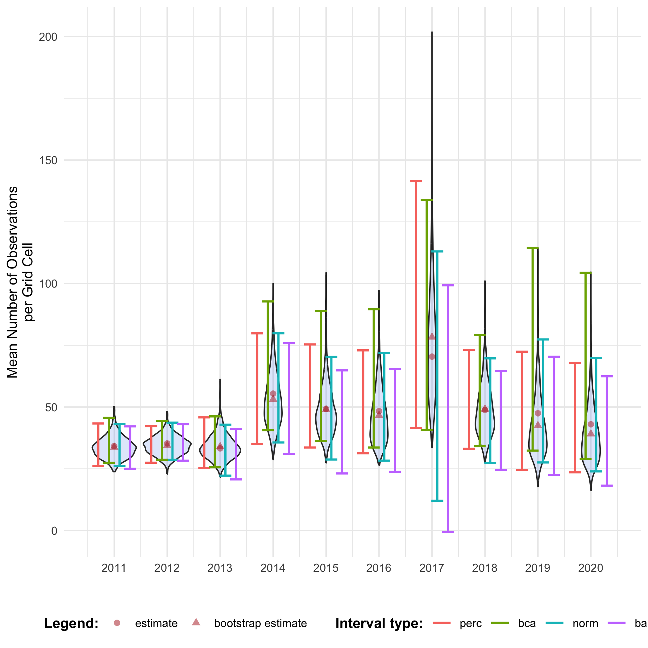

Confidence intervals for mean number of occurrences over time.

See the visualising temporal trends tutorial for information on which interval types should be calculated and/or reported and how temporal trends can be visualised.

Advanced usage of `calculate_bootstrap_ci()`

Comparison with a reference group

As discussed in the bootstrap tutorial, we can also compare indicator values to a reference group. In time series analyses, this often means comparing each year’s indicator to a baseline year (e.g., the first or last year in the series). To do this, we perform bootstrapping over the difference between indicator values. This process yields bootstrap replicate distributions of differences in indicator values.

bootstrap_results_ref <- bootstrap_cube(
  data_cube = processed_cube,
  fun = mean_obs,
  grouping_var = "year",
  samples = 1000,
  ref_group = 2011,
  seed = 123
)

head(bootstrap_results_ref)
#>   sample year est_original   rep_boot  est_boot  se_boot  bias_boot
#> 1      1 2012     1.094245  8.1881078 0.6583191 5.475053 -0.4359261
#> 2      2 2012     1.094245  7.6061946 0.6583191 5.475053 -0.4359261
#> 3      3 2012     1.094245 -4.6058908 0.6583191 5.475053 -0.4359261
#> 4      4 2012     1.094245  2.4102039 0.6583191 5.475053 -0.4359261
#> 5      5 2012     1.094245  6.2626545 0.6583191 5.475053 -0.4359261
#> 6      6 2012     1.094245 -0.1577162 0.6583191 5.475053 -0.4359261

If the BCa interval is calculated and a reference group is used, jackknifing is implemented differently. Consider $\hat{\theta} = \hat{\theta}_1 - \hat{\theta}_2$ where $\hat{\theta}_1$ is the estimate for the indicator value of a non-reference period (sample size $n_1$) and $\hat{\theta}_2$ is the estimate for the indicator value of a reference period (sample size $n_2$). The acceleration is now calculated as follows:

$$ \hat{a} = \frac{1}{6} \frac{\sum_{i = 1}^{n_1 + n_2}(I_i^3)}{\left( \sum_{i = 1}^{n_1 + n_2}(I_i^2) \right)^{3/2}} $$

$I_i$ can be calculated using the negative or positive jackknife. Such that

$\hat{\theta}{-i} = \hat{\theta}{1,-i} - \hat{\theta}_2 \text{ for } i = 1, \ldots, n_1$, and

$\hat{\theta}{-i} = \hat{\theta}{1} - \hat{\theta}_{2,-i} \text{ for } i = n_1 + 1, \ldots, n_1 + n_2$

Therefore, if you want to calculate the BCa intervals using calculate_bootstrap_ci(), you also need to provide ref_group = 2011.

#> Warning in norm_inter(h(t), adj_alpha): Extreme order statistics used as endpoints.
#> Warning in norm_inter(h(t), adj_alpha): Extreme order statistics used as endpoints.

ci_mean_obs_ref %>%
  filter(int_type == "bca") %>%
  head()
#>   year est_original    est_boot   se_boot  bias_boot int_type conf         ll       ul
#> 1 2012    1.0942452  0.65831911  5.475053 -0.4359261      bca 0.95 -10.762164 11.04344
#> 2 2013   -0.9219589 -0.07108256  6.690590  0.8508764      bca 0.95 -12.851385 13.06589
#> 3 2014   21.2638321 19.32958556 10.982093 -1.9342466      bca 0.95   5.818720 57.17064
#> 4 2015   15.0697689 14.80578656 10.723767 -0.2639823      bca 0.95   2.503933 58.08685
#> 5 2016   14.1628569 13.30622198 12.131657 -0.8566350      bca 0.95  -1.755266 52.49345
#> 6 2017   36.2442462 43.13141123 23.943155  6.8871650      bca 0.95   7.190653 96.55713

We see that the mean number of observations is higher in some years compared to 2011. Because the BCa intervals are above 0 in 2014, 2015, 2017 and 2018, we might even say it is significant for those years. This will be further explored in the effect classification tutorial.

# Make interval type factor
ci_mean_obs_ref <- ci_mean_obs_ref %>%
  mutate(
    int_type = factor(
      int_type, levels = c("perc", "bca", "norm", "basic")
    )
  )

# Get bias vales
bias_mean_obs <- bootstrap_results_ref %>%
  distinct(year, estimate = est_original, `bootstrap estimate` = est_boot)

# Get estimate values
estimate_mean_obs <- bias_mean_obs %>%
  pivot_longer(cols = c("estimate", "bootstrap estimate"),
               names_to = "Legend", values_to = "value") %>%
  mutate(Legend = factor(Legend, levels = c("estimate", "bootstrap estimate"),
                         ordered = TRUE))
# Visualise
bootstrap_results_ref %>%
  ggplot(aes(x = year)) +
  # Distribution
  geom_violin(aes(y = rep_boot, group = year),
              fill = alpha("cornflowerblue", 0.2)) +
  # Estimates and bias
  geom_point(data = estimate_mean_obs, aes(y = value, shape = Legend),
             colour = "firebrick", size = 2, alpha = 0.5) +
  # Intervals
  geom_errorbar(data = ci_mean_obs_ref,
                aes(ymin = ll, ymax = ul, colour = int_type),
                position = position_dodge(0.8), linewidth = 0.8) +
  # Settings
  labs(y = "Mean Number of Observations\nper Grid Cell Compared to 2011",
       x = "", shape = "Legend:", colour = "Interval type:") +
  scale_x_continuous(breaks = sort(unique(bootstrap_results_ref$year))) +
  theme_minimal() +
  theme(legend.position = "bottom",
        legend.title = element_text(face = "bold"))
#> Warning: Using shapes for an ordinal variable is not advised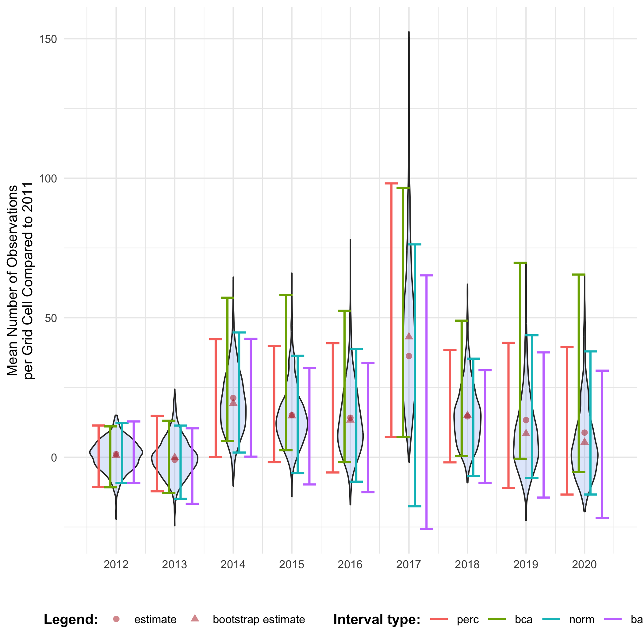

Confidence intervals for mean number of occurrences over time (ref).

Note that the choice of the reference year should be well considered. Keep in mind which comparisons should be made, and what the motivation is behind the reference period. A high or low value in the reference period relative to other periods, e.g. an exceptional bad or good year, can affect the magnitude and direction of the calculated differences. Whether this should be avoided or not, depends on the motivation behind the choice and the research question. A reference period can be determined by legislation, or by the start of a monitoring campaign. A specific research question can determine the periods that need to be compared. Furthermore, the variability of the estimate of reference period affects the width of confidence intervals for the differences. A more variable reference period will propagate greater uncertainty. In the case of GBIF data, more data will be available in recent years than in earlier years. If this is the case, it could make sense to select the last period as a reference period. In a way, this also avoids the arbitrariness of choice for the reference period. You compare previous situations with the current situation (last year), where you could repeat this comparison annually, for example. Finally, when comparing multiple indicators, we recommend using a consistent reference period to maintain comparability

Transformations

Consider the calculation of Pielou’s evenness on a random subset of the data from 2011-2015. We take only a small subset of the dataset and we artificially create a community with high evenness. This is an indicator that has values between 0 and 1. Higher evenness values indicate a more balanced community (a value of 1 means that all species are equally abundant), while low values indicate a more unbalanced community (a value of 0 means that one species dominates completely).

set.seed(123)

# Make dataset smaller
rows <- sample(nrow(bird_cube_belgium), 1000)
bird_cube_belgium_even <- bird_cube_belgium[rows, ]

# Make dataset even
bird_cube_belgium_even$n <- rnbinom(nrow(bird_cube_belgium_even),
                                    size = 2, mu = 100)

# Process cube
processed_cube_even <- process_cube(
  bird_cube_belgium_even,
  first_year = 2011,
  last_year = 2015,
  cols_occurrences = "n"
)

We create a custom function to calculate evenness:

calc_evenness <- function(data) {
  data %>%
    # Calculate number of observations
    dplyr::group_by(year, scientificName) %>%
    dplyr::summarise(obs = sum(obs), .groups = "drop_last") %>%
    # Calculate evenness by year
    dplyr::mutate(
      tot = sum(obs),
      p = obs / tot,
      p_ln_p = p * log(p),
      ln_S = log(dplyr::n_distinct(scientificName)),
      diversity_val = (-sum(p_ln_p)) / ln_S
    ) %>%
    dplyr::ungroup() %>%
    # Get distinct values
    dplyr::distinct(year, diversity_val)
}

We perform bootstrapping as before. Note that you can also perform bootstrapping of processed_cube_even using the b3gbi function pielou_evenness_ts().

bootstrap_results_evenness <- bootstrap_cube(
  data_cube = processed_cube_even,
  fun = calc_evenness,
  grouping_var = "year",
  samples = 1000,
  seed = 123
)

We calculate the percentile, BCa, normal and basic intervals with calculate_bootstrap_ci(). We get a warning message for BCa calculation because we are using a relatively small dataset.

ci_evenness <- calculate_bootstrap_ci(
  bootstrap_samples_df = bootstrap_results_evenness,
  grouping_var = "year",
  type = c("perc", "bca", "norm", "basic"),
  data_cube = processed_cube_even,
  fun = calc_evenness
)
#> Warning in norm_inter(h(t), adj_alpha): Extreme order statistics used as endpoints.
#> Warning in norm_inter(h(t), adj_alpha): Extreme order statistics used as endpoints.
#> Warning in norm_inter(h(t), adj_alpha): Extreme order statistics used as endpoints.
#> Warning in norm_inter(h(t), adj_alpha): Extreme order statistics used as endpoints.
#> Warning in norm_inter(h(t), adj_alpha): Extreme order statistics used as endpoints.

# Make interval type factor
ci_evenness <- ci_evenness %>%
  mutate(
    int_type = factor(
      int_type, levels = c("perc", "bca", "norm", "basic")
    )
  )

# Get bias vales
bias_mean_obs <- bootstrap_results_evenness %>%
  distinct(year, estimate = est_original, `bootstrap estimate` = est_boot)

# Get estimate values
estimate_mean_obs <- bias_mean_obs %>%
  pivot_longer(cols = c("estimate", "bootstrap estimate"),
               names_to = "Legend", values_to = "value") %>%
  mutate(Legend = factor(Legend, levels = c("estimate", "bootstrap estimate"),
                         ordered = TRUE))
# Visualise
bootstrap_results_evenness %>%
  ggplot(aes(x = year)) +
  # Distribution
  geom_violin(aes(y = rep_boot, group = year),
              fill = alpha("cornflowerblue", 0.2)) +
  # Estimates and bias
  geom_point(data = estimate_mean_obs, aes(y = value, shape = Legend),
             colour = "firebrick", size = 2, alpha = 0.5) +
  # Intervals
  geom_errorbar(data = ci_evenness,
                aes(ymin = ll, ymax = ul, colour = int_type),
                position = position_dodge(0.8), linewidth = 0.8) +
  # Settings
  labs(y = "Evenness", x = "", shape = "Legend:", colour = "Interval type:") +
  scale_x_continuous(breaks = sort(unique(bootstrap_results_evenness$year))) +
  theme_minimal() +
  theme(legend.position = "bottom",
        legend.title = element_text(face = "bold"))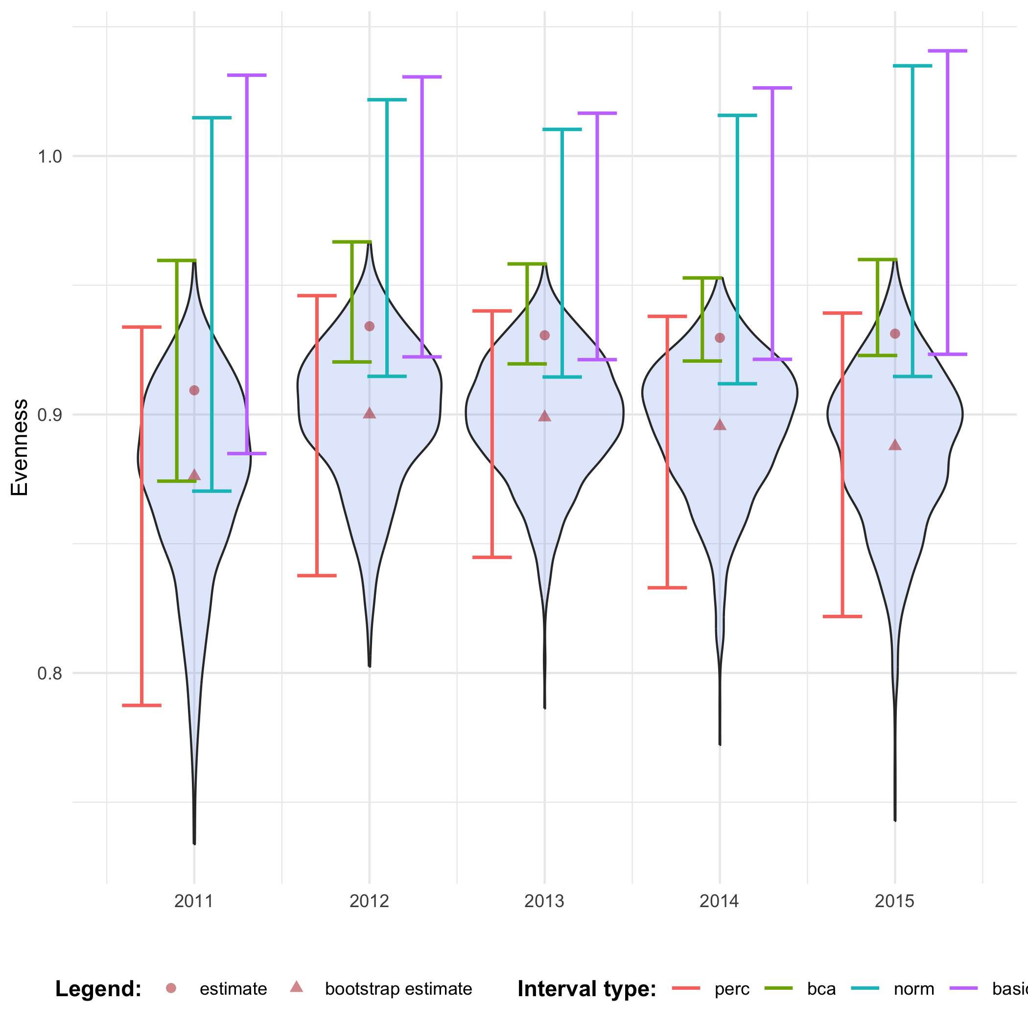
#> Warning: Using shapes for an ordinal variable is not advised

Confidence intervals for evenness over time.

We notice that the normal and basic intervals have limits larger than 1 which is an impossible value for evenness. This is because their intervals are symmetrical around $\hat{\theta} - \text{Bias}_{\text{boot}}$. We can use transformation functions to account for this. The intervals are calculated on the scale of h and the inverse function hinv are applied to the resulting intervals. For values between 0 and 1, we can use the logit function and its inverse:

# Logit transformation
logit <- function(p) {
  log(p / (1 - p))
}

# Inverse logit transformation
inv_logit <- function(l) {
  exp(l) / (1 + exp(l))
}

We enter them through calculate_bootstrap_ci().

ci_evenness_trans <- calculate_bootstrap_ci(
  bootstrap_samples_df = bootstrap_results_evenness,
  grouping_var = "year",
  type = c("perc", "bca", "norm", "basic"),
  h = logit,
  hinv = inv_logit,
  data_cube = processed_cube_even,
  fun = calc_evenness
)
#> Warning in norm_inter(h(t), adj_alpha): Extreme order statistics used as endpoints.
#> Warning in norm_inter(h(t), adj_alpha): Extreme order statistics used as endpoints.
#> Warning in norm_inter(h(t), adj_alpha): Extreme order statistics used as endpoints.
#> Warning in norm_inter(h(t), adj_alpha): Extreme order statistics used as endpoints.
#> Warning in norm_inter(h(t), adj_alpha): Extreme order statistics used as endpoints.

# Make interval type factor
ci_evenness_trans <- ci_evenness_trans %>%
  mutate(
    int_type = factor(
      int_type, levels = c("perc", "bca", "norm", "basic")
    )
  )

# Get bias vales
bias_mean_obs <- bootstrap_results_evenness %>%
  distinct(year, estimate = est_original, `bootstrap estimate` = est_boot)

# Get estimate values
estimate_mean_obs <- bias_mean_obs %>%
  pivot_longer(cols = c("estimate", "bootstrap estimate"),
               names_to = "Legend", values_to = "value") %>%
  mutate(Legend = factor(Legend, levels = c("estimate", "bootstrap estimate"),
                         ordered = TRUE))
# Visualise
bootstrap_results_evenness %>%
  ggplot(aes(x = year)) +
  # Distribution
  geom_violin(aes(y = rep_boot, group = year),
              fill = alpha("cornflowerblue", 0.2)) +
  # Estimates and bias
  geom_point(data = estimate_mean_obs, aes(y = value, shape = Legend),
             colour = "firebrick", size = 2, alpha = 0.5) +
  # Intervals
  geom_errorbar(data = ci_evenness_trans,
                aes(ymin = ll, ymax = ul, colour = int_type),
                position = position_dodge(0.8), linewidth = 0.8) +
  # Settings
  labs(y = "Evenness", x = "", shape = "Legend:", colour = "Interval type:") +
  scale_y_continuous(limits = c(NA, 1)) +
  scale_x_continuous(breaks = sort(unique(bootstrap_results_evenness$year))) +
  theme_minimal() +
  theme(legend.position = "bottom",
        legend.title = element_text(face = "bold"))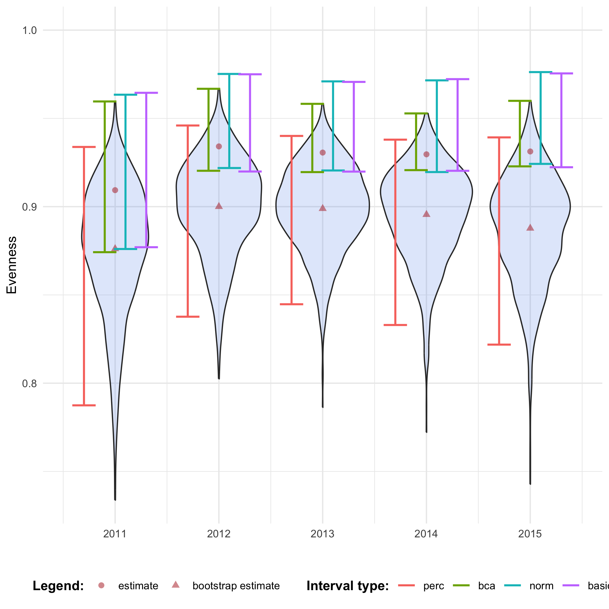
#> Warning: Using shapes for an ordinal variable is not advised

Now we see that all the intervals fall within the expected range.

Issues with bias correction for species richness indicators

Consider the calculation of observed species richness on the same subset used in the previous subsection. We create a custom function to calculate richness:

calc_richness <- function(data) {
  data %>%
    dplyr::group_by(year) %>%
    dplyr::summarise(diversity_val = n_distinct(scientificName),
                     .groups = "drop")
}

We perform bootstrapping as before. Note that you can also perform bootstrapping of processed_cube_small using the b3gbi function obs_richness_ts(). In this case, a group-specific bootstrap would be more appropriate, but for the sake of simplicity we stick to the whole-cube bootstrap here. For a detailed discussion of when to use each approach, see this tutorial.

bootstrap_results_richness <- bootstrap_cube(
  data_cube = processed_cube_even,
  fun = calc_richness,
  grouping_var = "year",
  samples = 1000,
  seed = 123
)

We calculate the percentile, BCa, normal and basic intervals with calculate_bootstrap_ci(). We get a warning message for BCa calculation. The bias is infinite such that the BCa intervals cannot be calculated.

ci_richness <- calculate_bootstrap_ci(
  bootstrap_samples_df = bootstrap_results_richness,
  grouping_var = "year",
  type = c("perc", "bca", "norm", "basic"),
  data_cube = processed_cube_even,
  fun = calc_richness
)
#> Warning in bca_ci(t0 = unique(df$est_original), t = df$rep_boot, a = a, : Estimated adjustment 'z0'
#> is infinite.
#> Warning in bca_ci(t0 = unique(df$est_original), t = df$rep_boot, a = a, : Estimated adjustment 'z0'
#> is infinite.
#> Warning in bca_ci(t0 = unique(df$est_original), t = df$rep_boot, a = a, : Estimated adjustment 'z0'
#> is infinite.
#> Warning in bca_ci(t0 = unique(df$est_original), t = df$rep_boot, a = a, : Estimated adjustment 'z0'
#> is infinite.
#> Warning in bca_ci(t0 = unique(df$est_original), t = df$rep_boot, a = a, : Estimated adjustment 'z0'
#> is infinite.

We notice that none of the intervals cover the estimate. The percentile interval does not account for bias, the BCa interval cannot be calculated because the bias is too large and the normal and basic intervals have overcompensated because of the large bootstrap bias.

# Make interval type factor
ci_richness <- ci_richness %>%
  mutate(
    int_type = factor(
      int_type, levels = c("perc", "bca", "norm", "basic")
    )
  )

# Get bias vales
bias_mean_obs <- bootstrap_results_richness %>%
  distinct(year, estimate = est_original, `bootstrap estimate` = est_boot)

# Get estimate values
estimate_mean_obs <- bias_mean_obs %>%
  pivot_longer(cols = c("estimate", "bootstrap estimate"),
               names_to = "Legend", values_to = "value") %>%
  mutate(Legend = factor(Legend, levels = c("estimate", "bootstrap estimate"),
                         ordered = TRUE))
# Visualise
bootstrap_results_richness %>%
  ggplot(aes(x = year)) +
  # Distribution
  geom_violin(aes(y = rep_boot, group = year),
              fill = alpha("cornflowerblue", 0.2)) +
  # Estimates and bias
  geom_point(data = estimate_mean_obs, aes(y = value, shape = Legend),
             colour = "firebrick", size = 2, alpha = 0.5) +
  # Intervals
  geom_errorbar(data = ci_richness,
                aes(ymin = ll, ymax = ul, colour = int_type),
                position = position_dodge(0.8), linewidth = 0.8) +
  # Settings
  labs(y = "Observed species richness", x = "", shape = "Legend:",
       colour = "Interval type:") +
  scale_x_continuous(breaks = sort(unique(bootstrap_results_richness$year))) +
  theme_minimal() +
  theme(legend.position = "bottom",
        legend.title = element_text(face = "bold"))
#> Warning: Using shapes for an ordinal variable is not advised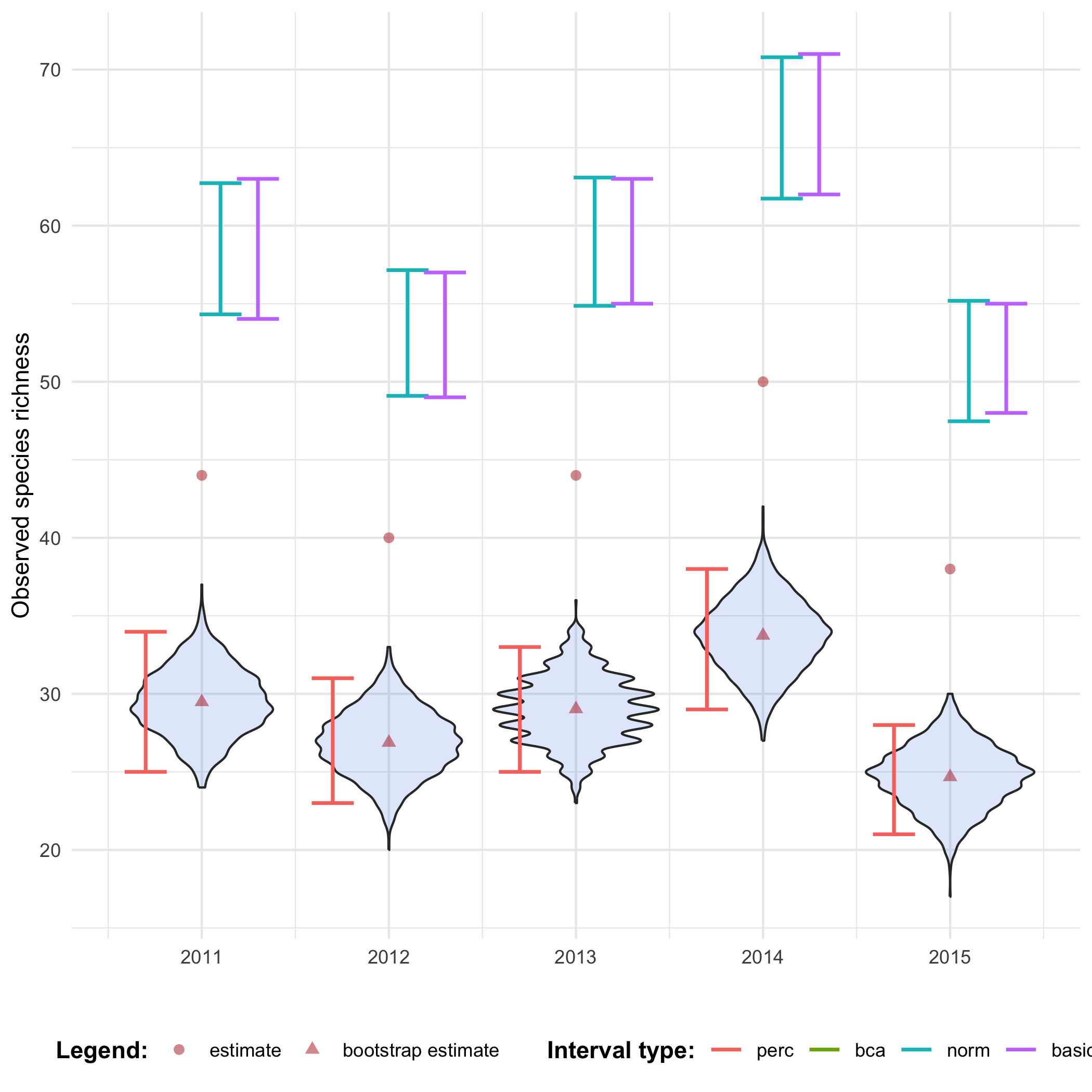

Confidence intervals for richness over time.

This issue arises because bootstrap resampling cannot introduce new species that were not present in the original sample (Dixon, 2001, p. 287). As a result, the observed species richness — which is simply the count of unique species — tends to be negatively biased in bootstrap replicates. This leads to an extreme mismatch between the original estimate and the distribution of bootstrap replicates. In such cases, the BCa intervals may fail altogether (e.g., due to infinite bias correction factors), and other bootstrap intervals (normal, basic) may overcorrect.

There is an option within calculate_bootstrap_ci() to center the confidence limits around the original estimate (no_bias = TRUE). This means the bootstrap distribution is used to calculate confidence intervals, except for the bootstrap bias. While it may “solve” technical problems with interval calculation (like infinite or undefined corrections), it does so at the cost of ignoring bootstrap bias. This approach should only be used with caution and clear justification, such as when the bootstrap bias is known to be an artifact of a sampling limitation and not of the underlying data structure.

Because of this inherent limitation, alternative richness estimators that account for undetected species are preferred when uncertainty quantification is needed. The vegan (Oksanen et al., 2024) and iNEXT (Hsieh et al., 2016) R packages provide such estimators, including Chao, Jackknife, and coverage-based rarefaction/extrapolation, all of which are designed to handle unseen species and provide meaningful uncertainty estimates.

Some of these estimators are also implemented directly for occurrence cubes in recent versions of b3gbi (≥ v0.4.0), offering integration into existing cube-based workflows. However, it is important to note that these are alternative estimators — they are not equivalent to observed richness and will yield different values by design.

ci_richness_no_bias <- calculate_bootstrap_ci(
  bootstrap_samples_df = bootstrap_results_richness,
  grouping_var = "year",
  type = c("perc", "bca", "norm", "basic"),
  no_bias = TRUE,
  data_cube = processed_cube_even,
  fun = calc_richness
)

Indeed, the intervals are now centered around the original estimate.

# Make interval type factor
ci_richness_no_bias <- ci_richness_no_bias %>%
  mutate(
    int_type = factor(
      int_type, levels = c("perc", "bca", "norm", "basic")
    )
  )

# Get bias vales
bias_mean_obs <- bootstrap_results_richness %>%
  distinct(year, estimate = est_original, `bootstrap estimate` = est_boot)

# Get estimate values
estimate_mean_obs <- bias_mean_obs %>%
  pivot_longer(cols = c("estimate", "bootstrap estimate"),
               names_to = "Legend", values_to = "value") %>%
  mutate(Legend = factor(Legend, levels = c("estimate", "bootstrap estimate"),
                         ordered = TRUE))
# Visualise
bootstrap_results_richness %>%
  ggplot(aes(x = year)) +
  # Distribution
  geom_violin(aes(y = rep_boot, group = year),
              fill = alpha("cornflowerblue", 0.2)) +
  # Estimates and bias
  geom_point(data = estimate_mean_obs, aes(y = value, shape = Legend),
             colour = "firebrick", size = 2, alpha = 0.5) +
  # Intervals
  geom_errorbar(data = ci_richness_no_bias,
                aes(ymin = ll, ymax = ul, colour = int_type),
                position = position_dodge(0.8), linewidth = 0.8) +
  # Settings
  labs(y = "Observed species richness", x = "", shape = "Legend:",
       colour = "Interval type:") +
  scale_x_continuous(breaks = sort(unique(bootstrap_results_richness$year))) +
  theme_minimal() +
  theme(legend.position = "bottom",
        legend.title = element_text(face = "bold"))
#> Warning: Using shapes for an ordinal variable is not advised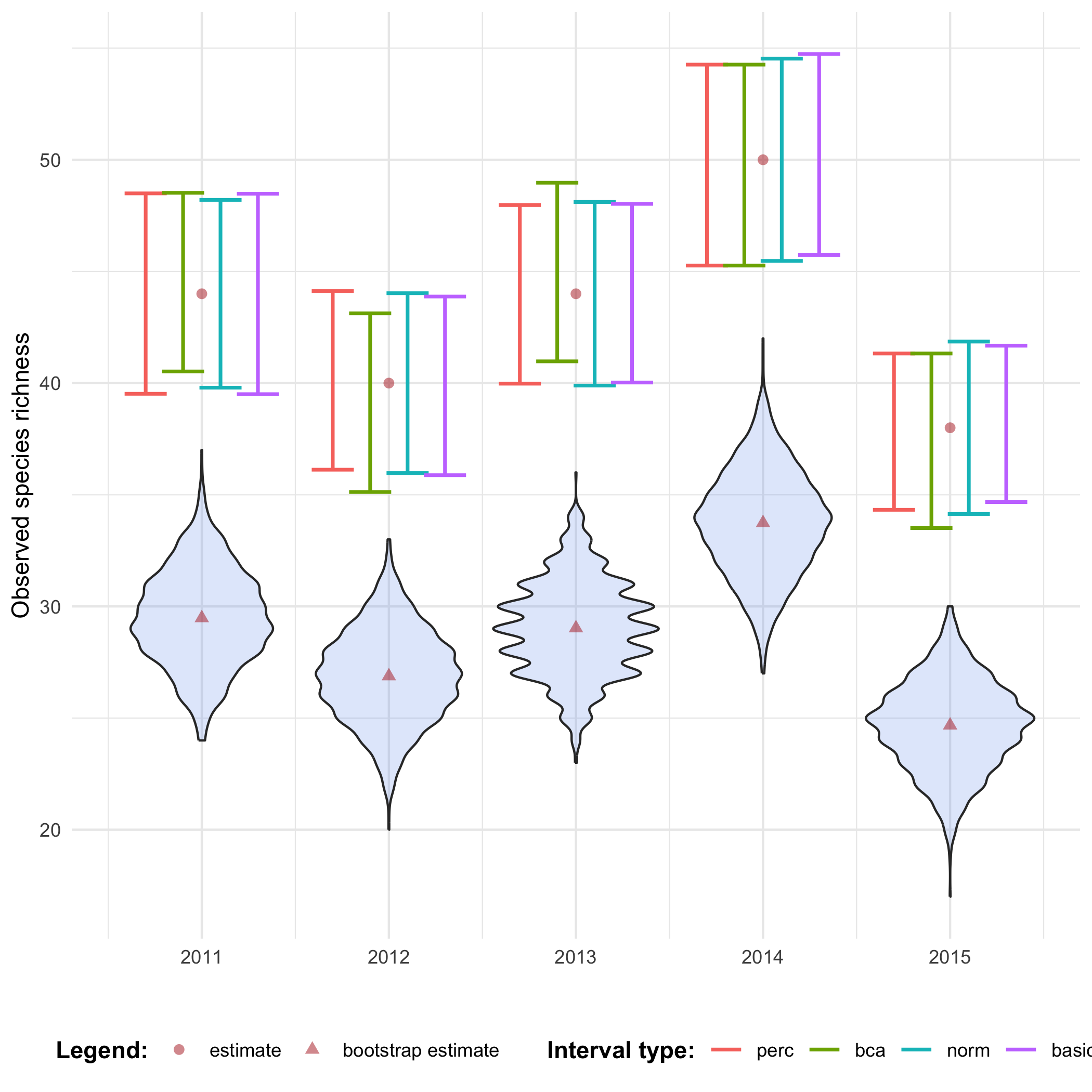

References

Canty, A., & Ripley, B. (1999). boot: Bootstrap Functions (Originally by Angelo Canty for S) [Computer software]. https://CRAN.R-project.org/package=boot

Davison, A. C., & Hinkley, D. V. (1997). Bootstrap Methods and their Application (1st ed.). Cambridge University Press. https://doi.org/10.1017/CBO9780511802843

DiCiccio, T. J., & Efron, B. (1996). Bootstrap confidence intervals. Statistical Science, 11(3). https://doi.org/10.1214/ss/1032280214

Dixon, P. M. (2001). The Bootstrap and the Jackknife: Describing the Precision of Ecological Indices. In S. M. Scheiner & J. Gurevitch (Eds.), Design and Analysis of Ecological Experiments (Second Edition, pp. 267–288). Oxford University PressNew York, NY. https://doi.org/10.1093/oso/9780195131871.003.0014

Efron, B. (1987). Better Bootstrap Confidence Intervals. Journal of the American Statistical Association, 82(397), 171–185. https://doi.org/10.1080/01621459.1987.10478410

Frangos, C. C., & Schucany, W. R. (1990). Jackknife estimation of the bootstrap acceleration constant. Computational Statistics & Data Analysis, 9(3), 271–281. https://doi.org/10.1016/0167-9473(90)90109-U

Calculating bootstrap confidence intervals

Introduction