Group-level sensitivity analysis

Introduction

When working with biodiversity data cubes, understanding how sensitive your indicators are to individual groups (like species, sites, or time periods) can be crucial for robust analysis. This tutorial introduces the cross_validate_cube() function from dubicube, which helps assess how individual categories influence biodiversity indicators using cross-validation.

Group-level cross-validation for data cubes

Cross-validation is a resampling technique commonly used in statistics and machine learning to evaluate model performance. In the context of biodiversity data cubes, we adapt cross-validation to assess how robust indicators are to the inclusion or exclusion of specific groups. This helps identify influential categories that disproportionately affect indicator values.

A data cube and a statistic

Consider a data cube $\mathbf{X}$ from which we want to calculate a statistic $\theta$. The data cube can be grouped, e.g. by taxon, that contains multiple categories, e.g. species1, species2, species3 …

Original Sample Data: $\mathbf{X} = {X_{11}, X_{12}, X_{13}, \ldots, X_{sn}}$
- The initial set of data points, where there are $s$ different categories in a group (e.g. $s = 10$ species in group taxon) and $n$ total samples across all categories (= the sample size). $n$ corresponds to the number of cells in a data cube or the number of rows in tabular format.
Statistic of Interest: $\theta$
- The parameter or statistic being estimated, such as the mean $\bar{X}$, variance $\sigma^2$, or a biodiversity indicator. Let $\hat{\theta}$ denote the estimated value of $\theta$ calculated from the complete dataset $\mathbf{X}$.

Resampling and recalculating

From $\mathbf{X}$, multiple data cubes $\mathbf{X}{-s_j}$ are created where in each new dataset a different category is removed compared to the original data cube $\mathbf{X}$. For example in dataset 1, species1 is excluded; in dataset 2 species2; in dataset 3 species3; and so on. For each new dataset, the statistic $\theta$ is again calculated: $\hat{\theta}{-s_j}$.

Cross-Validation (CV) Sample: $\mathbf{X}_{-s_j}$
- The full dataset $\mathbf{X}$ excluding all samples belonging to category $j$. This subset is used to investigate the influence of category $j$ on the estimated statistic $\hat{\theta}$.
CV Estimate for Category $\mathbf{j}$: $\hat{\theta}_{-s_j}$
- The value of the statistic of interest calculated from $\mathbf{X}{-s_j}$, which excludes category $j$. For example, if $\theta$ is the sample mean, $\hat{\theta}{-s_j} = \bar{X}_{-s_j}$.

Derivation of error measures

From this, we can calculate different error measures that help inform further analyses or decision-making steps.

Error Measures:
- The Error is the difference between the statistic estimated without category $j$ ($\hat{\theta}_{-s_j}$) and the statistic calculated on the complete dataset ($\hat{\theta}$).

$$ \text{Error}{s_j} = \hat{\theta}{-s_j} - \hat{\theta} $$

The Relative Error is the absolute error, normalized by the true estimate $\hat{\theta}$ and a small error term $\epsilon = 10^{-8}$ to avoid division by zero.

$$ \text{Rel. Error}{s_j} = \frac{|\hat{\theta}{-s_j} - \hat{\theta}|}{\hat{\theta} +\epsilon} $$

The Percent Error is the relative error expressed as a percentage.

$$ \text{Perc. Error}{s_j} = \text{Rel. Error}{s_j} \times 100 % $$

Summary Measures:
- The Mean Relative Error (MRE) is the average of the relative errors over all categories.

$$ \text{MRE} = \frac{1}{s} \sum_{j=1}^s \text{Rel. Error}_{s_j} $$

The Mean Squared Error (MSE) is the average of the squared errors.

$$ \text{MSE} = \frac{1}{s} \sum_{j=1}^s (\text{Error}_{s_j})^2 $$

The Root Mean Squared Error (RMSE) is the square root of the MSE.

$$ \text{RMSE} = \sqrt{\text{MSE}} $$

Getting started with dubicube

Our method can be used on any dataframe from which a statistic is calculated and a grouping variable is present. For this tutorial, we focus on occurrence cubes. Therefore, we will use the b3gbi package for processing the raw data before we go over to the cross-validation.

# Load packages
library(dubicube)

# Data loading and processing
library(frictionless) # Load example datasets
library(b3gbi)        # Process occurrence cubes

# General
library(ggplot2)      # Data visualisation
library(dplyr)        # Data wrangling

Loading and processing the data

We load the bird cube data from the b3data data package using frictionless (see also here). It is an occurrence cube for birds in Belgium between 2000 en 2024 using the MGRS grid at 10 km scale.

# Read data package
b3data_package <- read_package(
  "https://zenodo.org/records/15211029/files/datapackage.json"
)

# Load bird cube data
bird_cube_belgium <- read_resource(b3data_package, "bird_cube_belgium_mgrs10")
head(bird_cube_belgium)
#> # A tibble: 6 × 8
#>    year mgrscode specieskey species           family           n mincoordinateuncertaintyinmeters familycount
#>   <dbl> <chr>         <dbl> <chr>             <chr>        <dbl>                            <dbl>       <dbl>
#> 1  2000 31UDS65     2473958 Perdix perdix     Phasianidae      1                             3536      261414
#> 2  2000 31UDS65     2474156 Coturnix coturnix Phasianidae      1                             3536      261414
#> 3  2000 31UDS65     2474377 Fulica atra       Rallidae         5                             1000      507437
#> 4  2000 31UDS65     2475443 Merops apiaster   Meropidae        6                             1000        1655
#> 5  2000 31UDS65     2480242 Vanellus vanellus Charadriidae     1                             3536      294808
#> 6  2000 31UDS65     2480637 Accipiter nisus   Accipitridae     1                             3536      855924

We process the cube with b3gbi. We select the data from 2011 - 2020.

processed_cube <- process_cube(
  bird_cube_belgium,
  first_year = 2011,
  last_year = 2020,
  cols_occurrences = "n"
)
processed_cube
#>
#> Processed data cube for calculating biodiversity indicators
#>
#> Date Range: 2011 - 2020
#> Single-resolution cube with cell size 10km ^2
#> Number of cells: 379
#> Grid reference system: mgrs
#> Coordinate range:
#>    xmin    xmax    ymin    ymax
#>  280000  710000 5480000 5700000
#>
#> Total number of observations: 13225290
#> Number of species represented: 646
#> Number of families represented: 92
#>
#> Kingdoms represented: Data not present
#>
#> First 10 rows of data (use n = to show more):
#>
#> # A tibble: 280,184 × 13
#>     year cellCode taxonKey scientificName      family       obs minCoordinateUncerta…¹ familyCount xcoord ycoord utmzone hemisphere resolution
#>    <dbl> <chr>       <dbl> <chr>               <chr>      <dbl>                  <dbl>       <dbl>  <dbl>  <dbl>   <int> <chr>      <chr>
#>  1  2011 31UDS65   2474051 Alectoris rufa      Phasianid…     1                    100      261414 460000 5.65e6      31 N          10km
#>  2  2011 31UDS65   2474377 Fulica atra         Rallidae       6                   1000      507437 460000 5.65e6      31 N          10km
#>  3  2011 31UDS65   2474831 Rallus aquaticus    Rallidae       1                   1000      507437 460000 5.65e6      31 N          10km
#>  4  2011 31UDS65   2478523 Picus viridis       Picidae        5                   3536      403587 460000 5.65e6      31 N          10km
#>  5  2011 31UDS65   2480242 Vanellus vanellus   Charadrii…     4                   1000      294808 460000 5.65e6      31 N          10km
#>  6  2011 31UDS65   2480332 Pluvialis apricaria Charadrii…     1                   1000      294808 460000 5.65e6      31 N          10km
#>  7  2011 31UDS65   2480482 Circus aeruginosus  Accipitri…     2                   3536      855924 460000 5.65e6      31 N          10km
#>  8  2011 31UDS65   2480487 Circus cyaneus      Accipitri…     9                   3536      855924 460000 5.65e6      31 N          10km
#>  9  2011 31UDS65   2480537 Buteo buteo         Accipitri…     8                   3536      855924 460000 5.65e6      31 N          10km
#> 10  2011 31UDS65   2480637 Accipiter nisus     Accipitri…     9                   3536      855924 460000 5.65e6      31 N          10km
#> # ℹ 280,174 more rows
#> # ℹ abbreviated name: ¹minCoordinateUncertaintyInMeters

Analysis of the data

Let’s say we are interested in the mean number of observations per grid cell per year. We create a function to calculate this.

# Function to calculate statistic of interest
# Mean observations per grid cell per year
mean_obs <- function(data) {
  obs <- x <- NULL

  data %>%
    dplyr::mutate(x = mean(obs), .by = "cellCode") %>%
    dplyr::summarise(diversity_val = mean(x), .by = "year") %>%
    as.data.frame()
}

We get the following results:

mean_obs(processed_cube$data)
#>    year diversity_val
#> 1  2011      48.83864
#> 2  2012      48.27942
#> 3  2013      48.13675
#> 4  2014      47.82226
#> 5  2015      47.39197
#> 6  2016      47.32866
#> 7  2017      46.31520
#> 8  2018      45.87515
#> 9  2019      45.93329
#> 10 2020      44.98668

On their own, these values don’t tell us how reliable they are. Therefore, we perform leave-one-species-out cross-validation (LOSO-CV) to investigate the impact of included species on the calculation of these values.

Leave-one-species-out cross-validation

We use the cross_validate_cube() function to do this. It relies on the following arguments:

data_cube:
The input data, either as a processed data cube (from b3gbi::process_cube()), or simply the dataframe inside it (i.e. processed_cube$data). For faster computation, passing just the dataframe is recommended.
fun:
A user-defined function that computes the statistic(s) of interest from data_cube. This function should return a dataframe that includes a column named diversity_val, containing the statistic to evaluate.
grouping_var:
The column(s) used for grouping the output of fun(). For example, if fun() returns one value per year, use grouping_var = "year".
out_var:
The variable used to leave out one group at a time during cross-validation. The default is "taxonKey" (typically representing species), which results in leave-one-species-out cross-validation.
progress:
Logical flag to show a progress bar. Set to TRUE to enable progress reporting; default is FALSE.

cv_results <- cross_validate_cube(
  data_cube = processed_cube,
  fun = mean_obs,
  grouping_var = "year",
  out_var = "taxonKey"
)

head(cv_results)
#>   id_cv year taxonkey_out   rep_cv est_original       error     sq_error  abs_error    rel_error perc_error         mre        mse      rmse
#> 1     1 2011      2474051 48.85551     48.83864  0.01686866 0.0002845518 0.01686866 0.0003453959 0.03453959 0.001122516 0.03544285 0.1882627
#> 2     2 2011      2474377 48.49272     48.83864 -0.34592150 0.1196616847 0.34592150 0.0070829473 0.70829473 0.001122516 0.03544285 0.1882627
#> 3     3 2011      2474831 48.91447     48.83864  0.07583503 0.0057509524 0.07583503 0.0015527672 0.15527672 0.001122516 0.03544285 0.1882627
#> 4     4 2011      2478523 48.66861     48.83864 -0.17002678 0.0289091060 0.17002678 0.0034813989 0.34813989 0.001122516 0.03544285 0.1882627
#> 5     5 2011      2480242 48.56884     48.83864 -0.26979464 0.0727891466 0.26979464 0.0055242048 0.55242048 0.001122516 0.03544285 0.1882627
#> 6     6 2011      2480332 48.97265     48.83864  0.13401280 0.0179594315 0.13401280 0.0027439914 0.27439914 0.001122516 0.03544285 0.1882627

The RMSE is an average error measure we get for each year. It looks very similar over the years.

# Visualise mean errors
ggplot(cv_results, aes(x = as.factor(year))) +
  # Reference line
  geom_hline(yintercept = 0, colour = "black", linetype = "dashed") +
  # Plot RMSE
  geom_point(aes(y = rmse), colour = "red", size = 3) +
  # Settings
  labs(x = "", y = "RMSE") +
  theme_minimal()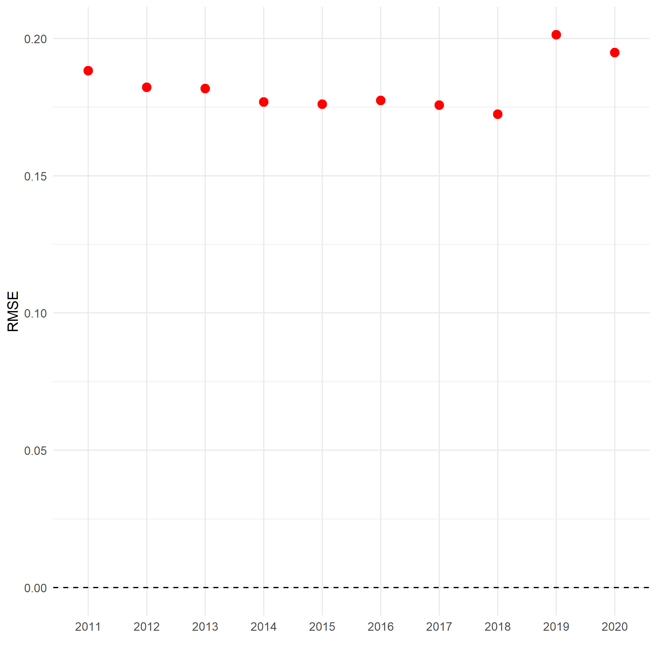

RMSE for mean number of occurrences over time.

Indeed, looking at the individual error values reveals similar patterns for every year. A species key 2481174 in year 2011 with error -2 means that without species 2481174, the average number of occurrences per grid cell would be 2 lower than the estimate based on the full dataset (in this case around 46.8 instead of 48.8).

# Get original estimates (based on full data cube)
original_estimates <- mean_obs(processed_cube$data)
original_estimates$label <- paste(
  "hat(theta) ==", round(original_estimates$diversity_val, 3)
)

# Visualise errors
ggplot(cv_results, aes(x = as.factor(year))) +
  # Reference line
  geom_hline(yintercept = 0, colour = "black", linetype = "dashed") +
  # Plot species keys
  geom_text(aes(y = error, colour = as.factor(taxonkey_out),
                label = as.factor(taxonkey_out))) +
  # Plot original estimates
  geom_label(data = original_estimates, aes(label = label),
             y = 0.9, parse = TRUE, size = 3) +
  # Settings
  scale_y_continuous(limits = c(NA, 1)) +
  labs(x = "", y = "LOSO-CV Error") +
  theme_minimal() +
  theme(legend.position = "")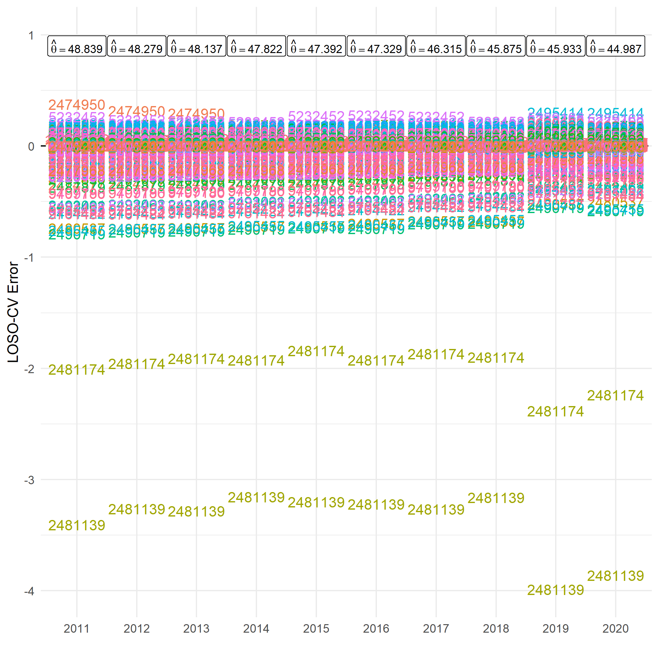

Species errors for mean number of occurrences over time.

There are two species that have a big effect on the calculation of our statistic.

2481174: Larus fuscus Linnaeus, 1758
2481139: Larus argentatus Pontoppidan, 1763

If we go back to the source of the data, we see that the data cube includes records from two large datasets strictly dedicated to these two species (2481174, 2481139).

index <- match("bird_cube_belgium_mgrs10", resources(b3data_package))
b3data_package$resources[[index]]$sources
#> [[1]]
#> [[1]]$title
#> [1] "GBIF Occurrence Download"
#>
#> [[1]]$path
#> [1] "https://doi.org/10.15468/dl.y3wpwk"

This suggests that the two species are overrepresented in the data cube, likely due to targeted monitoring efforts. Their disproportionate influence inflates indicator values, potentially distorting the true diversity signal. Group-level sensitivity analysis like this helps uncover such sampling biases, ensuring that biodiversity indicators better reflect ecological reality rather than data artifacts.

Advanced usage of `cross_validate_cube()`

Cross-validate simple dataframes

As stated in the documentation, it is also possible to cross-validate over a dataframe. In this case, set the argument processed_cube = FALSE. This is implemented allow for flexible use of simple dataframes, while still encouraging the use of b3gbi::process_cube() as default functionality.

cv_results_df <- cross_validate_cube(
  data_cube = processed_cube$data,      # data.frame object
  fun = mean_obs,
  grouping_var = "year",
  out_var = "taxonKey",
  processed_cube = FALSE
)

Optional arguments

The cross_validate_cube() function includes several optional parameters that give you more control over how the cross-validation is performed. These arguments are not required for basic use but can be helpful in specific scenarios.

Cross-validation Method: crossv_method
Determines how data is partitioned for cross-validation.
- "loo" (default):
  Leave-one-out cross-validation. One category in out_var (e.g. one species) is excluded at a time.
- "kfold":
  K-fold cross-validation. All categories in out_var are split into k subsets, and each subset is excluded once while the others are used for analysis.
  Note: this method is experimental and results should be interpreted with caution.
Number of Folds: k
Specifies the number of folds when using "kfold" cross-validation.
Default is 5. Only used when crossv_method = "kfold".
Maximum Number of Categories: max_out_cats
Sets an upper limit on the number of unique categories in out_var that will be excluded one-by-one during cross-validation.
Default is 1000. This helps prevent long runtimes for datasets with many unique categories. You can increase this if needed, but expect slower computation.