Introduction

gcube

The goal of gcube is to provide a simulation framework for biodiversity data cubes using the R programming language. This can start from simulating multiple species distributed in a landscape over a temporal scope. In a second phase, the simulation of a variety of observation processes and effort can generate actual occurrence datasets. Based on their (simulated) spatial uncertainty, occurrences can then be designated to a grid to form a data cube.

Simulation studies offer numerous benefits due to their ability to mimic real-world scenarios in controlled and customizable environments. Ecosystems and biodiversity data are very complex and involve a multitude of interacting factors. Simulations allow researchers to model and understand the complexity of ecological systems by varying parameters such as spatial and/or temporal clustering, species prevalence, etc.

Installation

Install gcube in R:

install.packages("gcube", repos = "https://b-cubed-eu.r-universe.dev")

You can install the development version from GitHub with:

# install.packages("remotes")
remotes::install_github("b-cubed-eu/gcube")

Package name rationale and origin story

The name gcube stands for “generate cube” since it can be used to generate biodiversity data cubes from minimal input. It was first developed during the hackathon “Hacking Biodiversity Data Cubes for Policy”, where it won the first price in the category “Visualization and training”. You can read the full story here: https://doi.org/10.37044/osf.io/vcyr7

Example

This is a basic example which shows the workflow for simulating a biodiversity data cube. It is divided in three steps or processes:

1. Occurrence process
2. Detection process
3. Grid designation process

The functions are set up such that a single polygon as input is enough to go through this workflow using default arguments. The user can change these arguments to allow for more flexibility.

# Load packages
library(gcube)

library(sf)      # working with spatial objects
library(dplyr)   # data wrangling
library(ggplot2) # visualisation with ggplot

We create a polygon as input. It represents the spatial extend of the species.

# Create a polygon to simulate occurrences within
polygon <- st_polygon(list(cbind(c(5, 10, 8, 2, 3, 5), c(2, 1, 7,9, 5, 2))))

# Visualise
ggplot() +
  geom_sf(data = polygon) +
  theme_minimal()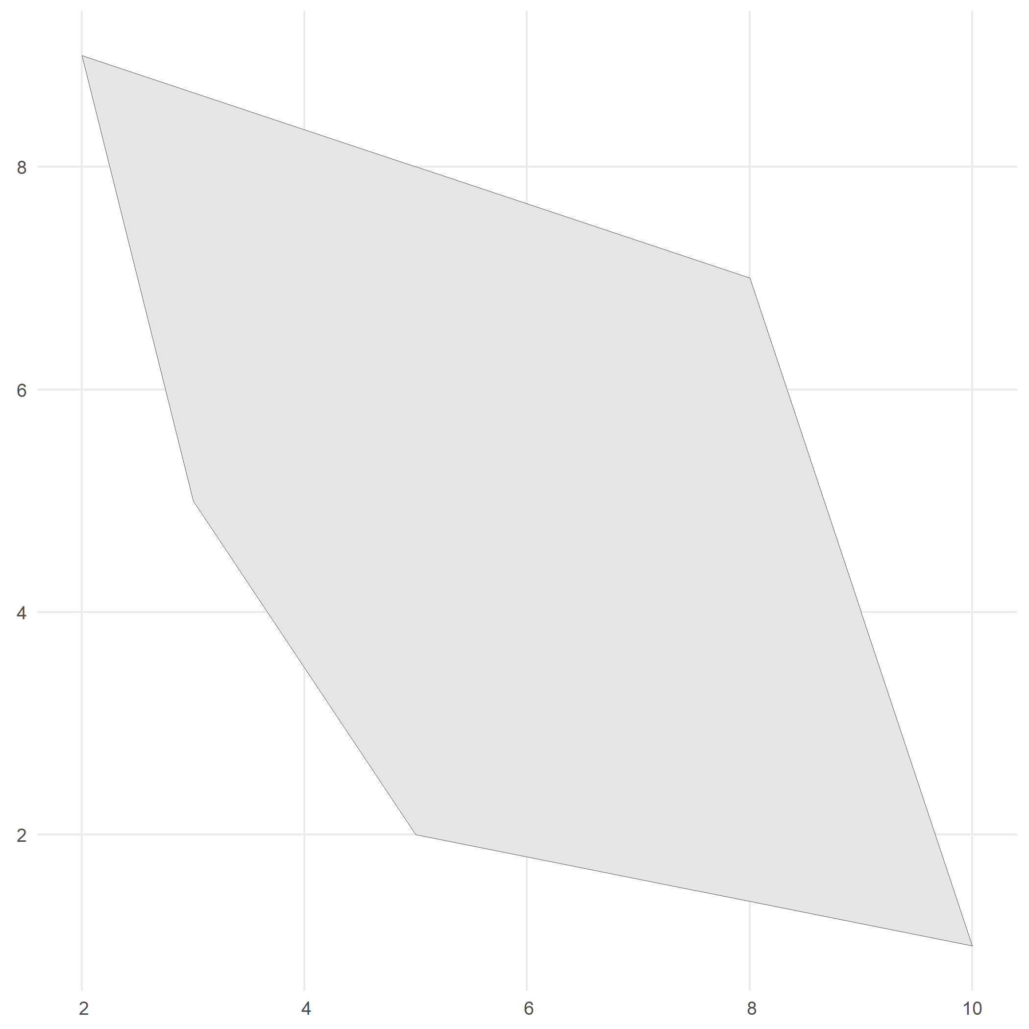

Occurrence process

We generate occurrence points within the polygon using the simulate_occurrences() function. In this function, the user can specify different levels of spatial clustering, and define the trend of number of occurrences over time. The default is a random spatial pattern and a single time point with rpois(1, 50) occurrences.

# Simulate occurrences within polygon
occurrences_df <- simulate_occurrences(
  species_range = polygon,
  initial_average_occurrences = 50,
  spatial_pattern = c("random", "clustered"),
  n_time_points = 1,
  seed = 123)
#> [using unconditional Gaussian simulation]

# Visualise
ggplot() +
  geom_sf(data = polygon) +
  geom_sf(data = occurrences_df) +
  theme_minimal()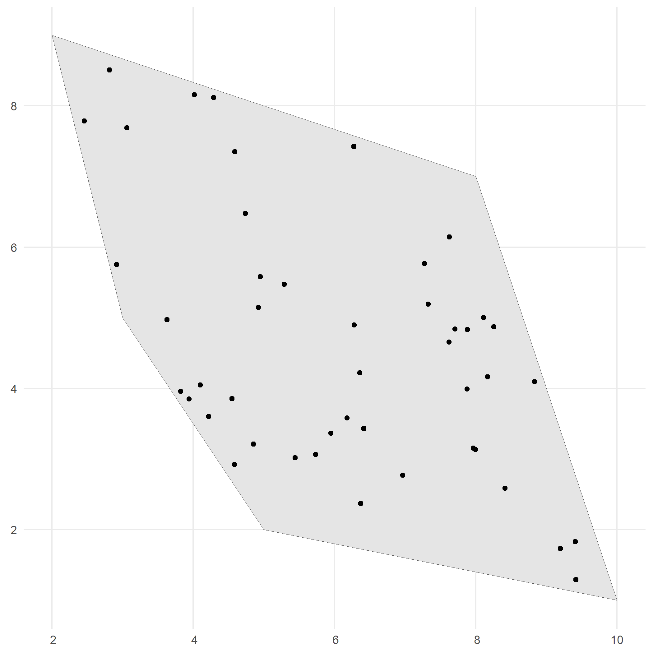

Detection process

In the second step we define the sampling process, based on the detection probability of the species and the sampling bias. This is done using the sample_observations() function. The default sampling bias is "no_bias", but bias can be added using a polygon or a grid as well.

# Detect occurrences
detections_df_raw <- sample_observations(
  occurrences = occurrences_df,
  detection_probability = 0.5,
  sampling_bias = c("no_bias", "polygon", "manual"),
  seed = 123)

# Visualise
ggplot() +
  geom_sf(data = polygon) +
  geom_sf(data = detections_df_raw,
          aes(colour = observed)) +
  theme_minimal()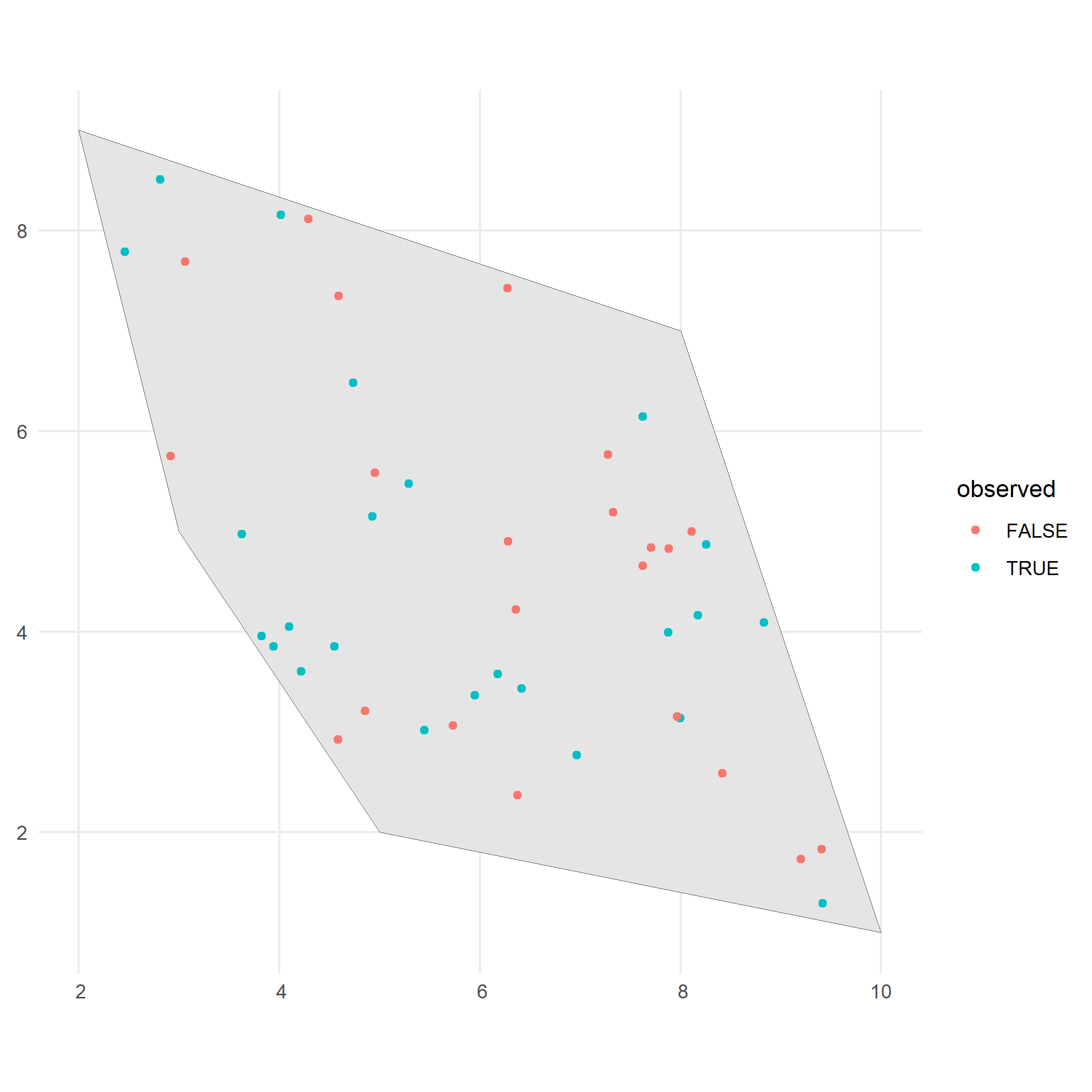

We select the detected occurrences and add an uncertainty to these observations. This can be done using the filter_observations() and add_coordinate_uncertainty() functions, respectively.

# Select detected occurrences only
detections_df <- filter_observations(
  observations_total = detections_df_raw)

# Add coordinate uncertainty
set.seed(123)
coord_uncertainty_vec <- rgamma(nrow(detections_df), shape = 2, rate = 6)
observations_df <- add_coordinate_uncertainty(
  observations = detections_df,
  coords_uncertainty_meters = coord_uncertainty_vec)

# Created and sf object with uncertainty circles to visualise
buffered_observations <- st_buffer(
  observations_df,
  observations_df$coordinateUncertaintyInMeters)

# Visualise
ggplot() +
  geom_sf(data = polygon) +
  geom_sf(data = buffered_observations,
          fill = alpha("firebrick", 0.3)) +
  geom_sf(data = observations_df, colour = "firebrick") +
  theme_minimal()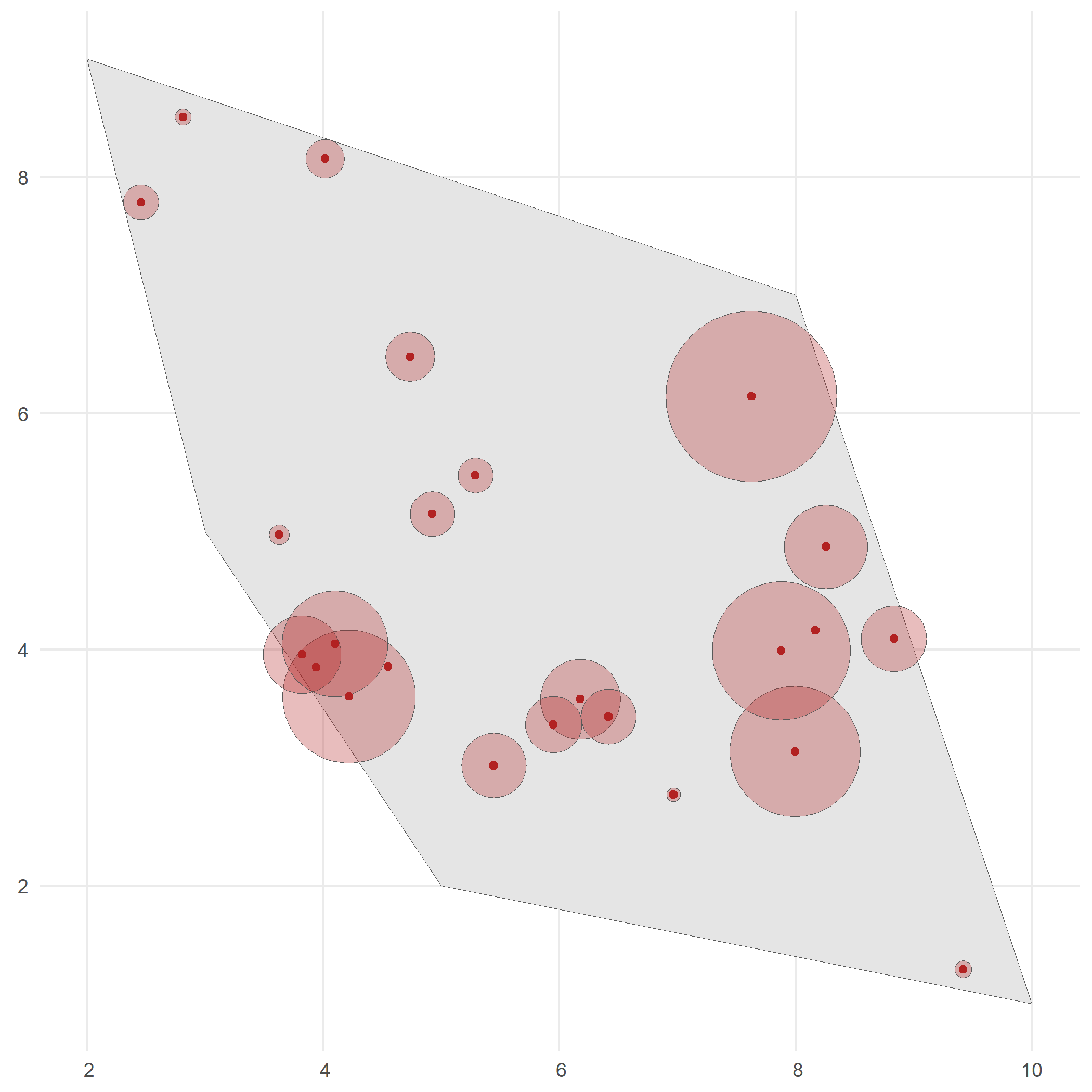

Grid designation process

Finally, observations are designated to a grid with grid_designation() to create an occurrence cube. We create a grid over the spatial extend using sf::st_make_grid().

# Define a grid over spatial extend
grid_df <- st_make_grid(
    buffered_observations,
    square = TRUE,
    cellsize = c(1.2, 1.2)
  ) %>%
  st_sf() %>%
  mutate(intersect = as.vector(st_intersects(geometry, polygon,
                                             sparse = FALSE))) %>%
  dplyr::filter(intersect == TRUE) %>%
  dplyr::select(-"intersect")

To create an occurrence cube, grid_designation() will randomly take a point within the uncertainty circle around the observations. These points can be extracted by setting the argument aggregate = FALSE.

# Create occurrence cube
occurrence_cube_df <- grid_designation(
  observations = observations_df,
  grid = grid_df,
  seed = 123)

# Get sampled points within uncertainty circle
sampled_points <- grid_designation(
  observations = observations_df,
  grid = grid_df,
  aggregate = FALSE,
  seed = 123)

# Visualise grid designation
ggplot() +
  geom_sf(data = occurrence_cube_df, linewidth = 1) +
  geom_sf_text(data = occurrence_cube_df, aes(label = n)) +
  geom_sf(data = buffered_observations,
          fill = alpha("firebrick", 0.3)) +
  geom_sf(data = sampled_points, colour = "blue") +
  geom_sf(data = observations_df, colour = "firebrick") +
  labs(x = "", y = "", fill = "n") +
  theme_minimal()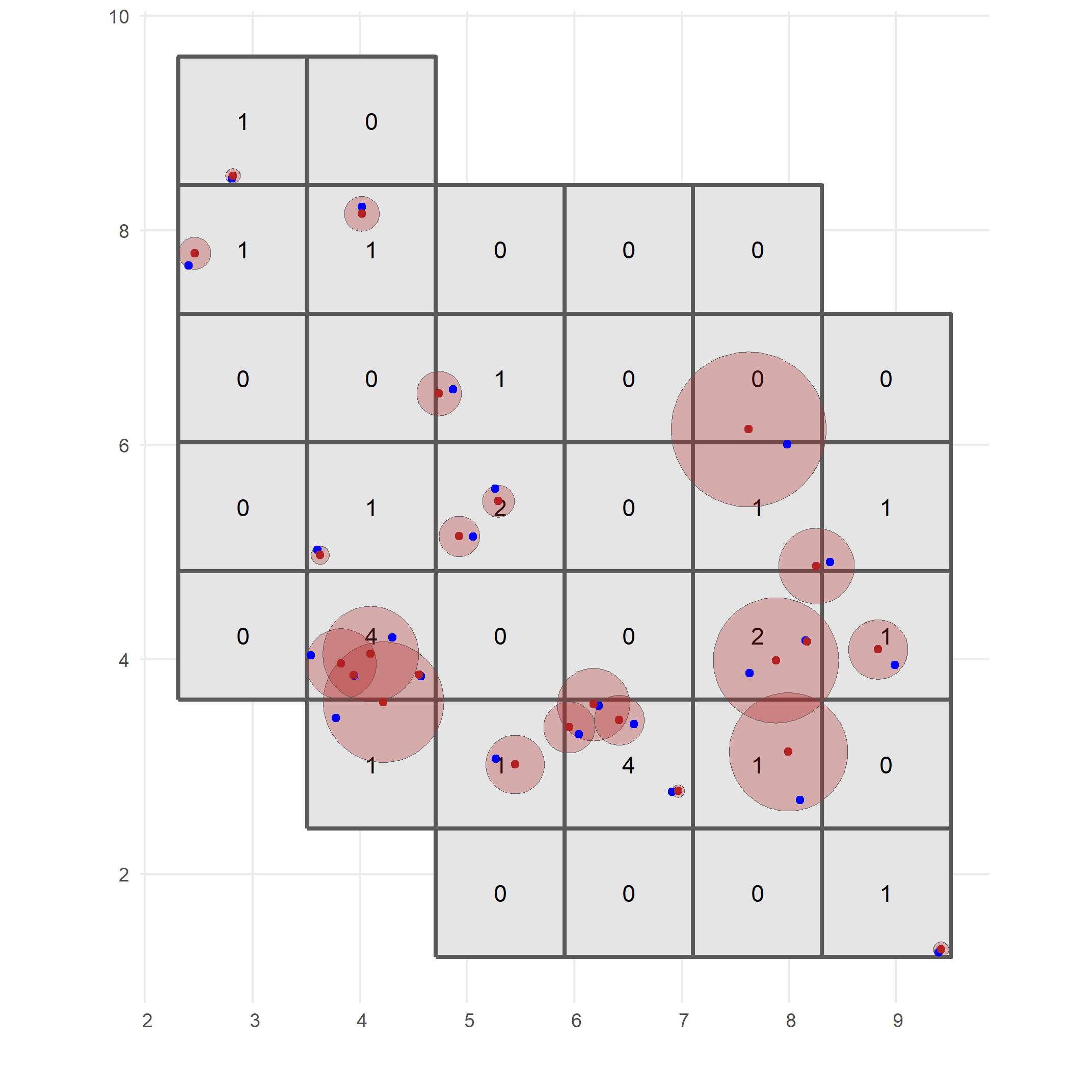

The output gives the number of observations per grid cell and minimal coordinate uncertainty per grid cell.

# Visualise minimal coordinate uncertainty
ggplot() +
  geom_sf(data = occurrence_cube_df, aes(fill = min_coord_uncertainty),
          alpha = 0.5, linewidth = 1) +
  geom_sf_text(data = occurrence_cube_df, aes(label = n)) +
  scale_fill_continuous(type = "viridis") +
  labs(x = "", y = "") +
  theme_minimal()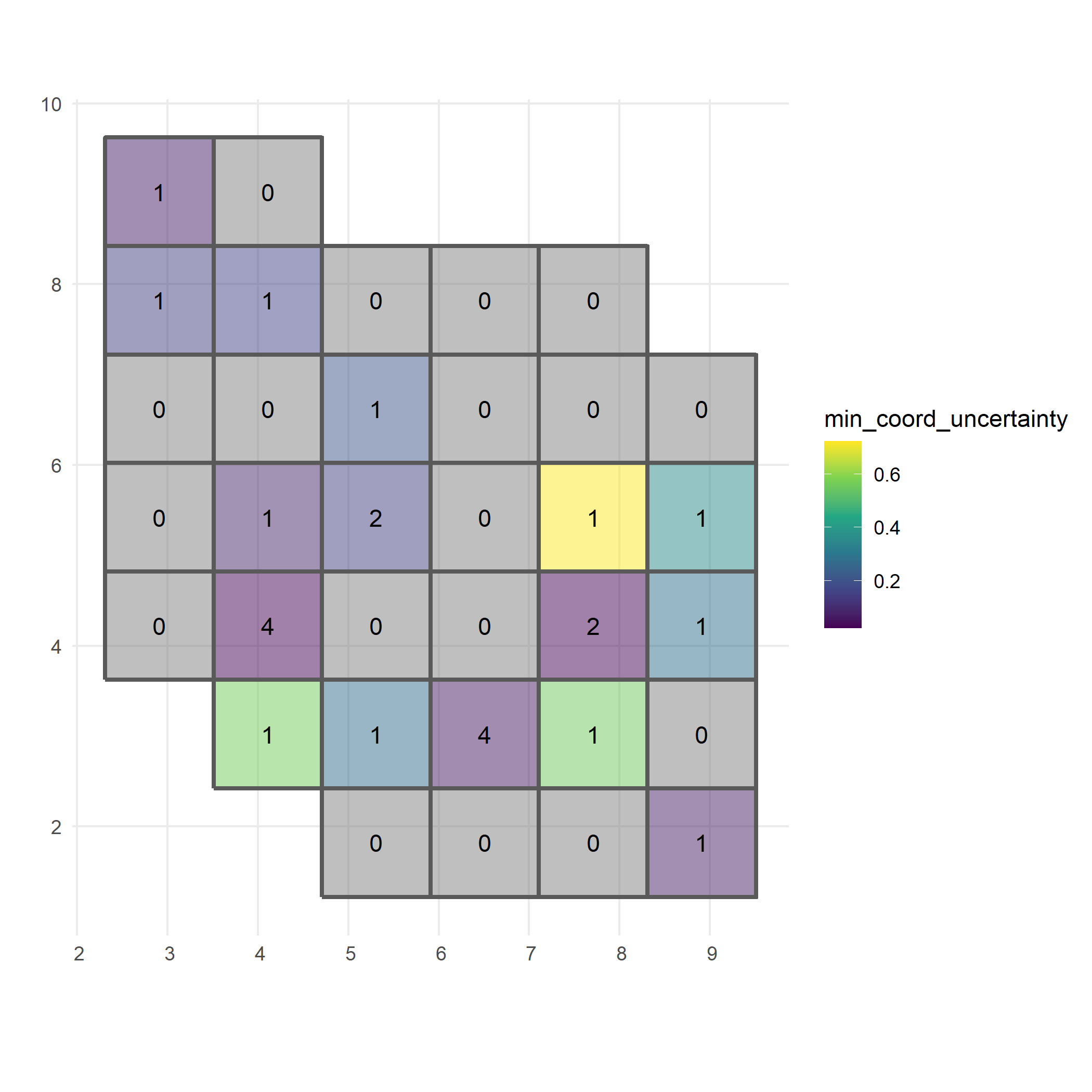

Cubes for multiple species

Each cube simulation function mentioned earlier has a corresponding mapping function. These mapping functions are designed to handle operations for multiple species simultaneously by using the purrr::pmap() function. Please consult the documentation for detailed information on how these mapping functions are implemented.

single species	multiple species
simulate_occurrences()	map_simulate_occurrences()
sample_observations()	map_sample_observations()
filter_observations()	map_filter_observations()
add_coordinate_uncertainty()	map_add_coordinate_uncertainty()
grid_designation()	map_grid_designation()