vscube: Virtual Suitability Cube
Species suitability refers to how favorable an environment is for a species to survive, reproduce, and grow in a specific area and time. It takes into account factors like climate, landscape, and resource availability.
Species Distribution Models (SDMs) are tools that use environmental and species occurrence data to study and predict the distribution of species across time and space. SDMs help identify suitable habitats, forecast the movements of invasive species, and illustrate how species distributions might change due to factors like climate change.
To facilitate the observation of suitability for multiple species over time and space, we developed a framework that uses Data Cubes, multidimensional arrays that organize data in a structured way. The goal of vscube is to outline the steps to create a stars object, which includes three dimensions: time, space (represented as grid cells), and species, with suitability as the main attribute. Stars objects can be sliced, aggregated along one of the dimensions, and analyzed, making them ideal for studying species suitability.
# install.packages("remotes")# remotes::install_github("b-cubed-eu/vscube")Download WorldClim predictors for May (Netherlands)
Section titled “Download WorldClim predictors for May (Netherlands)”The function vsc_build_worldclim() automatically downloads monthly climatic variables from WorldClim, builds a stars data cube for all 12 months, and extracts a SpatRaster with the selected month’s layers.
It returns a list with three elements:
-
$stars: astarscube with all variables and all months -
$predictors: aSpatRasterwith the selected month’s layers -
$vars_kept: a character vector with the successfully downloaded variables
In this example we build May (month = 5) climatic predictors for the Netherlands ("NLD").
# load packageslibrary(vscube)library(terra)library(stars)library(ggplot2)library(viridis)# Build climatic data for the Netherlands, Maycl_nld <- vsc_build_worldclim(iso3 = "NLD", month = 5)
# The function returns a list with three components:str(cl_nld, max.level = 1)#> List of 3#> $ stars :List of 5#> ..- attr(*, "dimensions")=List of 3#> .. ..- attr(*, "raster")=List of 4#> .. .. ..- attr(*, "class")= chr "stars_raster"#> .. ..- attr(*, "class")= chr "dimensions"#> ..- attr(*, "class")= chr "stars"#> $ predictors:S4 class 'SpatRaster' [package "terra"]#> $ vars_kept : chr [1:5] "tmin" "tmax" "prec" "tavg" ...# Show which variables were successfully downloadedcl_nld$vars_kept#> [1] "tmin" "tmax" "prec" "tavg" "wind"First output: SpatRaster with predictors
Section titled “First output: SpatRaster with predictors”terra::plot(cl_nld$predictors, col = viridis(100))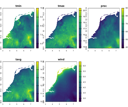
# Basic info about the predictorscl_nld$predictors#> class : SpatRaster#> size : 420, 540, 5 (nrow, ncol, nlyr)#> resolution : 0.008333333, 0.008333333 (x, y)#> extent : 3, 7.5, 50.5, 54 (xmin, xmax, ymin, ymax)#> coord. ref. : lon/lat WGS 84 (EPSG:4326)#> sources : NLD_wc2.1_30s_tmin.tif#> NLD_wc2.1_30s_tmax.tif#> NLD_wc2.1_30s_prec.tif#> ... and 2 more sources#> names : tmin, tmax, prec, tavg, wind#> min values : 5.5, 13.8, 39, 10, 2.7#> max values : 10.1, 20.4, 90, 15, 6.4#> time (raw) : 5names(cl_nld$predictors)#> [1] "tmin" "tmax" "prec" "tavg" "wind"terra::nlyr(cl_nld$predictors)#> [1] 5terra::ext(cl_nld$predictors)#> SpatExtent : 3, 7.5, 50.5, 54 (xmin, xmax, ymin, ymax)terra::crs(cl_nld$predictors)#> [1] "GEOGCRS[\"WGS 84\",\n ENSEMBLE[\"World Geodetic System 1984 ensemble\",\n MEMBER[\"World Geodetic System 1984 (Transit)\"],\n MEMBER[\"World Geodetic System 1984 (G730)\"],\n MEMBER[\"World Geodetic System 1984 (G873)\"],\n MEMBER[\"World Geodetic System 1984 (G1150)\"],\n MEMBER[\"World Geodetic System 1984 (G1674)\"],\n MEMBER[\"World Geodetic System 1984 (G1762)\"],\n MEMBER[\"World Geodetic System 1984 (G2139)\"],\n MEMBER[\"World Geodetic System 1984 (G2296)\"],\n ELLIPSOID[\"WGS 84\",6378137,298.257223563,\n LENGTHUNIT[\"metre\",1]],\n ENSEMBLEACCURACY[2.0]],\n PRIMEM[\"Greenwich\",0,\n ANGLEUNIT[\"degree\",0.0174532925199433]],\n CS[ellipsoidal,2],\n AXIS[\"geodetic latitude (Lat)\",north,\n ORDER[1],\n ANGLEUNIT[\"degree\",0.0174532925199433]],\n AXIS[\"geodetic longitude (Lon)\",east,\n ORDER[2],\n ANGLEUNIT[\"degree\",0.0174532925199433]],\n USAGE[\n SCOPE[\"Horizontal component of 3D system.\"],\n AREA[\"World.\"],\n BBOX[-90,-180,90,180]],\n ID[\"EPSG\",4326]]"# convert SpatRaster to data frame for ggplotdf_tmin <- terra::as.data.frame(cl_nld$predictors[["tmin"]], xy = TRUE, na.rm = TRUE)
ggplot(df_tmin, aes(x, y, fill = tmin)) + geom_raster() + coord_equal() + scale_fill_viridis_c(name = "°C", option = "viridis") + labs(title = "Minimum temperature (tmin) — May, Netherlands", x = NULL, y = NULL) + theme_minimal(base_size = 12) + theme(panel.grid = element_blank())#> Warning: Raster pixels are placed at uneven horizontal intervals and will be shifted#> ℹ Consider using `geom_tile()` instead.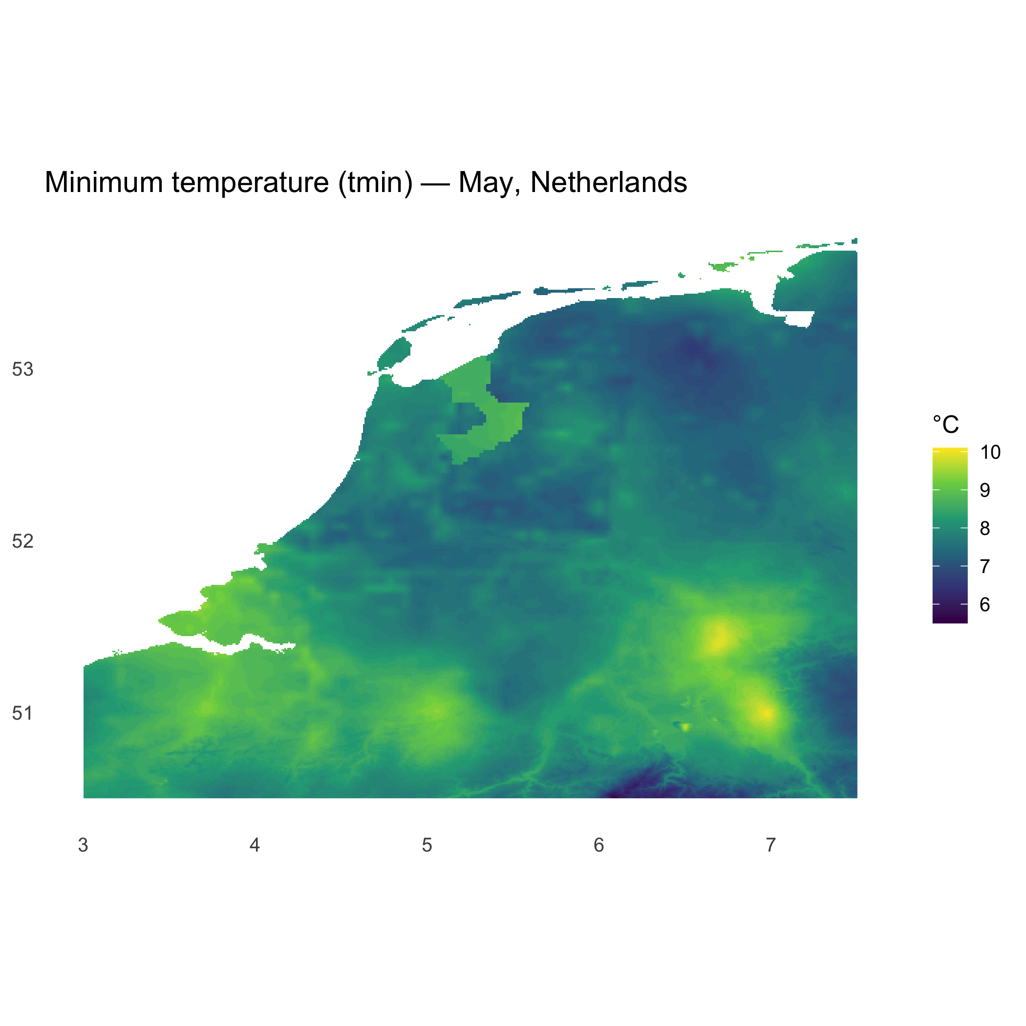
Second output: stars data cube
Section titled “Second output: stars data cube”A stars Data Cube with predictors as attributes and x, y, t as dimensions
# The full stars cube contains all 12 months for each variablecl_nld$stars#> stars object with 3 dimensions and 5 attributes#> attribute(s), summary of first 1e+05 cells:#>       Min. 1st Qu. Median         Mean 3rd Qu. Max.  NA's#> tmin  -0.8    -0.4   -0.1  0.007868939     0.2  2.6 63985#> tmax   3.7     4.3    4.6  4.718736640     5.0  6.4 63985#> prec  58.0    66.0   68.0 67.980036096    70.0 80.0 63985#> tavg   1.6     1.9    2.2  2.363004291     2.6  4.5 63985#> wind   4.0     4.6    5.2  5.363057057     6.0  7.8 63985#> dimension(s):#>      from  to offset     delta refsys point x/y#> x       1 540      3  0.008333 WGS 84 FALSE [x]#> y       1 420     54 -0.008333 WGS 84 FALSE [y]#> time    1  12      1         1     NA    NA
# Dimensions and attribute namesst_dimensions(cl_nld$stars)#>      from  to offset     delta refsys point x/y#> x       1 540      3  0.008333 WGS 84 FALSE [x]#> y       1 420     54 -0.008333 WGS 84 FALSE [y]#> time    1  12      1         1     NA    NAnames(cl_nld$stars)#> [1] "tmin" "tmax" "prec" "tavg" "wind"
Read and prepare occurrences
Section titled “Read and prepare occurrences”Together with climatic predictors, occurrences are needed: vsc_read_occurrences() ingests a GBIF TSV/TXT and returns a cleaned data frame with the key columns (scientificName, decimalLatitude, decimalLongitude, year) filtered by year range and removing NAs.
occ <- vsc_read_occurrences( example_file(), year_min = 2000, year_max = 2010 )head(occ)#> scientificName decimalLatitude decimalLongitude year#> 1 Anemone nemorosa L. 52.09306 6.27293 2007#> 2 Ophrys apifera Huds. 50.89106 5.92014 2010#> 3 Galium verum L. 53.43582 5.46957 2010#> 4 Galium verum L. 51.70893 5.94423 2000#> 5 Galium verum L. 51.65332 4.37782 2000#> 6 Galium verum L. 52.51377 6.55657 2000The example contains 5 species of flowers in Flanders.
Split occurrences by species
Section titled “Split occurrences by species”After reading and cleaning the GBIF dataset with vsc_read_occurrences(), we can divide it into separate species datasets using split_species_data().
This creates a list of data frames, one per species, that will be used in model training.
# split the data by species namesp_list <- split_species_data(occ)
# show list summarylength(sp_list)#> [1] 5names(sp_list)#> [1] "Anemone nemorosa L."             "Chrysosplenium alternifolium L."#> [3] "Galium verum L."                 "Ophrys apifera Huds."#> [5] "Paris quadrifolia L."
Train SDMs (MaxEnt) for multiple species
Section titled “Train SDMs (MaxEnt) for multiple species”The function vsc_create_sdm_for_species_list() trains a MaxEnt model for each species in your list (the output of split_species_data()), using a common stack of environmental predictors (e.g., the May predictors you built with vsc_build_worldclim()).
The function:
-
Cleans points (removes NAs, off-grid cells, duplicates per raster cell).
-
Samples background points.
-
Trains MaxEnt via
enmSdmX::trainMaxEnt()for each species.
Returns a list with:
-
$models: one trained model per species. -
$predictions: suitability rasters (SpatRaster) for the training area (one per species).
Note that this is not meant to have an ecological relevance: the purpose is to show the data cube structure with suitability values.
# Train MaxEnt for each species
sdms <- vsc_create_sdm_for_species_list(species_list = sp_list,stack_clima = cl_nld$predictors, # SpatRaster for the training area/monthbackground_points = 10000, # adjust as neededpredictors = names(cl_nld$predictors),verbose = TRUE)#> [vscube] Processing species: Anemone nemorosa L.#> [vscube] Processing species: Chrysosplenium alternifolium L.#> [vscube] Processing species: Galium verum L.#> [vscube] Processing species: Ophrys apifera Huds.#> [vscube] Processing species: Paris quadrifolia L.
# Inspect outputsnames(sdms)#> [1] "models"      "predictions"
names(sdms$models)[1:5]#> [1] "Anemone nemorosa L."             "Chrysosplenium alternifolium L."#> [3] "Galium verum L."                 "Ophrys apifera Huds."#> [5] "Paris quadrifolia L."
# Quick look at predictions (training area)terra::plot(terra::rast(sdms$predictions), col = mako(100))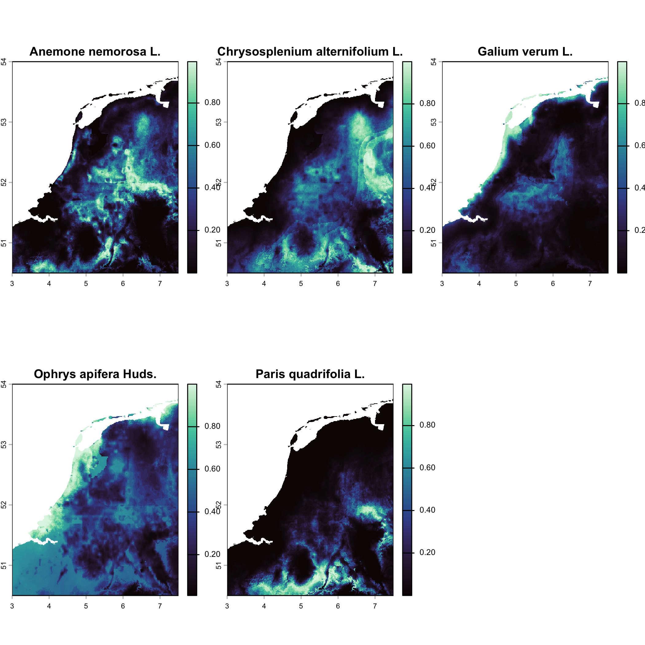
Project trained models to a new area (same month/variables)
Section titled “Project trained models to a new area (same month/variables)”What this does:
- Builds WorldClim predictors for the new target area (here: Belgium, May)
- Applies each traine model to the new predictor stack
- Returns a
starscube with attributesuitand dimensionspecies.
# Build predictors for the new area (Belgium, month = 5)cl_bel <- vsc_build_worldclim(iso3 = "BEL", month = 5)
# Optional sanity check: names must match the training predictorsstopifnot(setequal(names(cl_bel$predictors), names(cl_nld$predictors)))

# Predict: models (from previous chunk) -> new area predictorspred_bel <- vsc_predict_sdm_for_new_area(models = sdms$models,new_stack = cl_bel$predictors)#> [vscube] Predicting: Anemone nemorosa L.#> [vscube] Predicting: Chrysosplenium alternifolium L.#> [vscube] Predicting: Galium verum L.#> [vscube] Predicting: Ophrys apifera Huds.#> [vscube] Predicting: Paris quadrifolia L.
The 3 dimensions are: x, y and species.
# Inspect the stars outputpred_bel # stars object with attribute "suit"#> stars object with 3 dimensions and 1 attribute#> attribute(s):#> Min. 1st Qu. Median Mean 3rd Qu. Max. NA's#> suit 6.182086e-10 0.05560188 0.1902957 0.2611484 0.4240361 0.9996012 67380#> dimension(s):#> from to offset delta refsys values x/y#> x 1 480 2.5 0.008333 WGS 84 NULL [x]#> y 1 360 52 -0.008333 WGS 84 NULL [y]#> species 1 5 NA NA NA Anemone nemorosa L.,...,Paris quadrifolia L.Aggregate species suitability into a polygon grid
Section titled “Aggregate species suitability into a polygon grid”After predicting habitat suitability for each species over the new area (Belgium), we can summarize those high-resolution maps into a regular grid. This step serves three main purposes:
-
compression: reduces raster resolution so the cube becomes smaller and faster to analyze.
-
comparability: aligns all species to the same polygon grid, enabling cross-species or cell-wise analysis.
-
interpretability: each grid cell represents an “average suitability” over that polygon’s extent.
vsc_make_grid_over() automatically builds a polygon grid covering the raster extent. You can control either:
n = c(nx, ny): number of grid cells along x and y, or
cellsize = 0.1: fixed size in degrees.
Once the grid is created, aggregate_suitability() computes the mean suitability of each species within every polygon, producing a compact stars object with:
-
one attribute:
suitability, and -
two dimensions:
cell(grid polygon) andspecies
Finally, vsc_plot_raster_with_grid() overlays the grid on top of one predictor (e.g., tmin) so you can visually inspect the aggregation layout.
# Make a grid over the new area’s predictor extent (Belgium)# Option A: pick grid size via number of cells in x,y:grid_bel <- vsc_make_grid_over(cl_bel$predictors, n = c(50, 50))
# Option B (alternative): fixed cellsize in degrees (e.g. ~0.1°)grid_bel <- vsc_make_grid_over(cl_bel$predictors, cellsize = 0.1)
# Aggregate the species stars cube (pred_bel) over polygonsagg_bel <- aggregate_suitability(pred_bel, grid_bel, fun = mean)
# output:agg_bel#> stars object with 2 dimensions and 1 attribute#> attribute(s):#>                   Min.   1st Qu.    Median      Mean   3rd Qu.      Max.#> suitability  0.1219109 0.2703462 0.3399906 0.4100135 0.5544951 0.8361634#> dimension(s):#>          from   to refsys point#> geometry    1 1200 WGS 84 FALSE#> species     1    5     NA    NA#>                                                                 values#> geometry POLYGON ((2.5 49, 2.6 49,...,...,POLYGON ((6.4 51.9, 6.5 5...#> species                   Anemone nemorosa L.,...,Paris quadrifolia L.st_dimensions(agg_bel)#>          from   to refsys point#> geometry    1 1200 WGS 84 FALSE#> species     1    5     NA    NA#>                                                                 values#> geometry POLYGON ((2.5 49, 2.6 49,...,...,POLYGON ((6.4 51.9, 6.5 5...#> species                   Anemone nemorosa L.,...,Paris quadrifolia L.names(agg_bel)#> [1] "suitability"
# show a raster layer with the grid on topvsc_plot_raster_with_grid(cl_bel$predictors[[1]], grid_bel)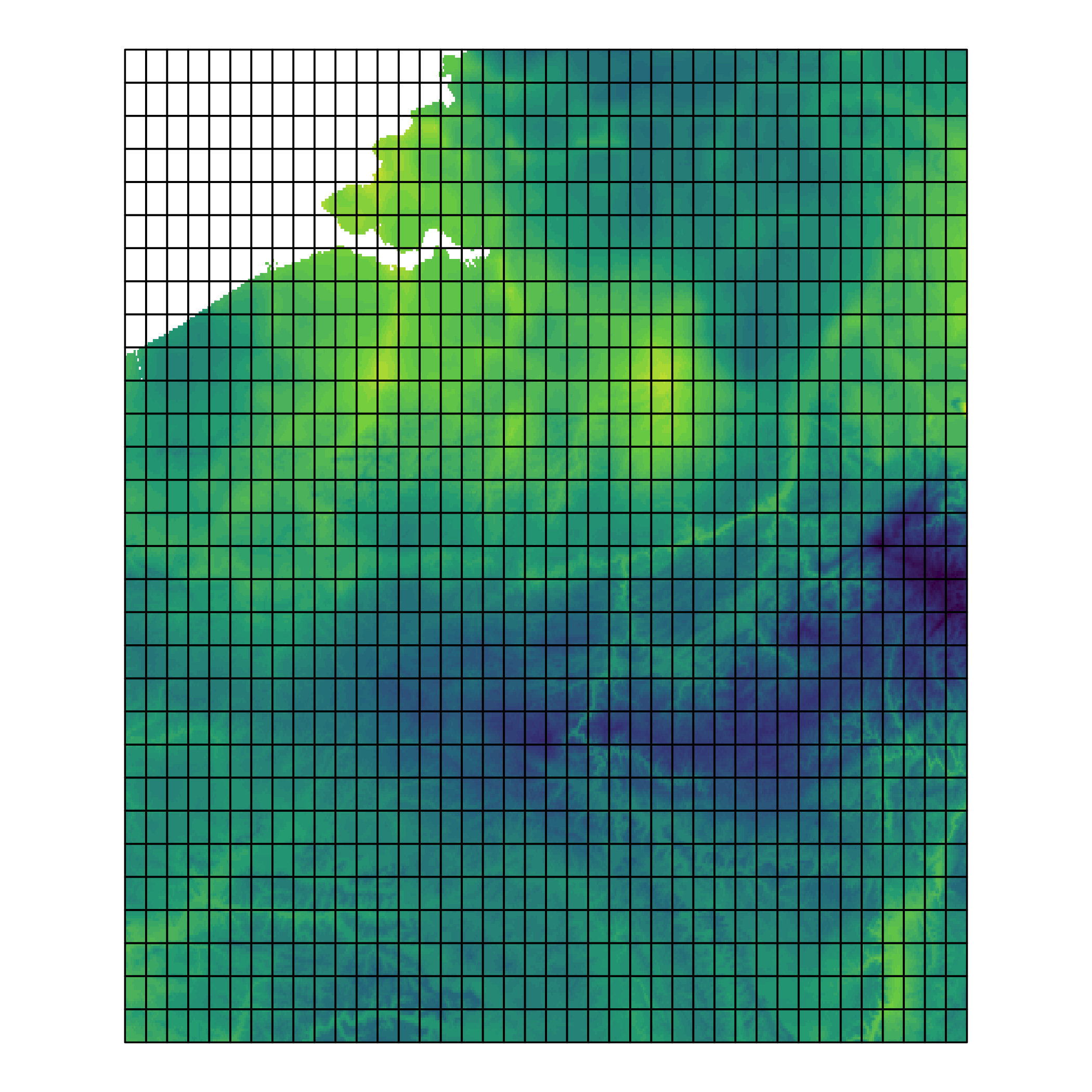
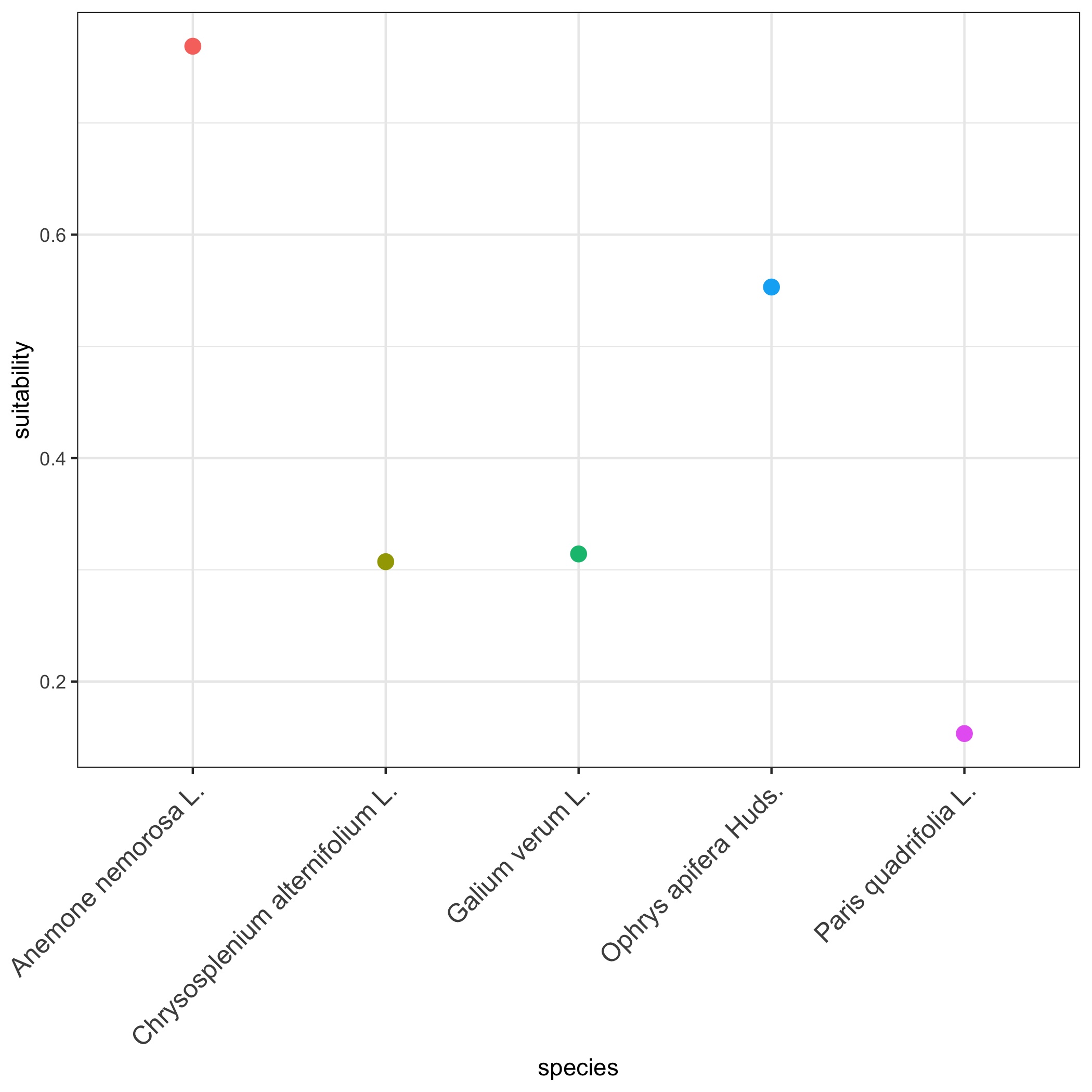
Inspect species suitability for a specific location
Section titled “Inspect species suitability for a specific location”Once the aggregated cube is ready, you can zoom in on a single grid cell — for example, the one containing Brussels — to see how all modeled species perform there.
This diagnostic step helps interpret local suitability patterns, identify species-rich vs. poor cells, and visually compare model outputs.
vsc_cell_id_for_point(): finds which polygon (cell) in the grid contains a given longitude–latitude coordinate. Then, vsc_cell_suitability_long() extracts all suitability values for that cell and reshapes them into a tidy long table with columns:
-
cell: polygon ID
-
species: species name
-
suitability: aggregated suitability value
vsc_plot_cell_suitability() plots these values as a quick bar or point chart, giving a visual “species profile” for that location.
This makes it easy to compare species’ modeled suitability within a single site or to rank locations by potential habitat richness.
# pick a point (Brussels)cell_id <- vsc_cell_id_for_point(grid_bel, lon = 4.3517, lat = 50.8503)
# extract long table of suitability per species for that celldf_long <- vsc_cell_suitability_long(agg_bel, cell_id)head(df_long)#>   cell                         species suitability#> 1  739             Anemone nemorosa L.   0.7686433#> 2  739 Chrysosplenium alternifolium L.   0.3072809#> 3  739                 Galium verum L.   0.3142103#> 4  739            Ophrys apifera Huds.   0.5531120#> 5  739            Paris quadrifolia L.   0.1534397
# Quick plot of species profile for this cellp_cell <- vsc_plot_cell_suitability(df_long)p_cell