
Step-by-step workflow
This vignette runs through a step-by-step workflow to visualise trait dispersion and assess species invasiveness and site invasibility. It begins with how to install and load invasimapr and outlines the (pre-)requisites for running the full workflow.
Install and load invasimapr
Section titled “Install and load invasimapr”Install* and load the invasimapr package from GitHub, ensuring all functions are available for use in the workflow.
# install.packages("remotes")# remotes::install_github("b-cubed-eu/invasimapr")
# If invasimapr is on CRAN:# install.packages("invasimapr")Load* the invasimapr package:
library(invasimapr)
if (!requireNamespace("invasimapr", quietly = TRUE)) {  knitr::knit_exit()}
# Optional: report package versionpackageVersion("invasimapr")#> [1] '0.2.0'
# Make sure all the functions are loaded# devtools::load_all() # alternative during local development
Load other R libraries
Section titled “Load other R libraries”Load core libraries for spatial processing, biodiversity modelling, and visualization required across the invasimapr analysis pipeline.
The workflow typically uses packages for:
- data manipulation (
dplyr,tidyr,purrr,tibble,stringr) - modelling (
glmmTMB,performance,MASS,glmnet,Matrix) - multivariate methods (
vegan,cluster) - spatial analysis (
sf) - visualisation (
ggplot2,viridis,pheatmap,factoextra)
For robust docs builds, we recommend not attaching large dependency sets with library() unless you will use them in this vignette. Instead, downstream vignettes should load what they need, and you can rely on pkg::fun() where practical.
Below is a light “availability check” that does not install anything.
# # Load essential packages# suppressPackageStartupMessages({#   need = c("dplyr","tidyr","purrr","tibble","stringr","ggplot2","Matrix","glmnet","rlang", "glmmTMB",#   "performance", "vegan", "cluster", "matrixStats", "sf", "MASS", "factoextra", "viridis", "pheatmap")#   to_install = need[!sapply(need, requireNamespace, quietly = TRUE)]#   if (length(to_install)) install.packages(to_install)#   lapply(need, library, character.only = TRUE)# })
deps = c(  # Core workflow  "dplyr","tidyr","purrr","tibble","stringr", "forcats",  "ggplot2",  # Modelling / stats  "glmmTMB","performance","Matrix","glmnet","MASS","vegan","cluster","matrixStats",  # Spatial  "sf",  # Viz helpers used in later steps  "viridis","pheatmap","factoextra")
is_installed = vapply(deps, requireNamespace, logical(1), quietly = TRUE)missing = deps[!is_installed]
cat("### Dependency check\n\n")if (length(missing) == 0) {  cat("- All recommended packages are available.\n")} else {  cat("- Missing packages (install before running the full workflow):\n")  cat(paste0("  - ", missing, collapse = "\n"), "\n")}
Data access and preparation
Section titled “Data access and preparation”Data access and preparation using dissmapr
Section titled “Data access and preparation using dissmapr”To acquire and prepare species occurrence data for biodiversity modelling using the dissmapr package, a series of modular functions streamline the workflow from raw observations to spatially aligned environmental predictors.
Install dissmapr
Section titled “Install dissmapr”Install and load the dissmapr package from GitHub, ensuring all functions are available for use in the workflow.
# # Install remotes if needed# install.packages("remotes")# remotes::install_github("b-cubed-eu/dissmapr")
# Ensure the package is loaded.# suppressWarnings() hides dissmapr's namespace-load import clashes# (intersect/union/time<-/aggregate from dplyr/terra/zoo/stats).ok <- suppressWarnings(suppressMessages(  requireNamespace("dissmapr", quietly = TRUE)))if (!ok) {  knitr::knit_exit()}# Optional: report package versionpackageVersion("dissmapr")#> [1] '0.2.0'
Import and harmonise biodiversity-occurrence data
Section titled “Import and harmonise biodiversity-occurrence data”The process begins with dissmapr::get_occurrence_data(), which imports biodiversity records, such as a GBIF butterfly dataset for South Africa, and harmonizes them into standardised formats. Input sources can include local CSV files, URLs, or zipped GBIF downloads. The function filters data by taxon and region, returning both raw records and site × species matrices in presence-absence or abundance form.
# Use local GBIF databfly_data = dissmapr::get_occurrence_data(  data = system.file("extdata", "gbif_butterflies.csv", package = "invasimapr"),  source_type = "local_csv",  sep = "\t")
# Check results but only a subset of columns to fit in consoledim(bfly_data)# str(bfly_data[,c(51,52,22,23,1,14,16,17,30)])head(bfly_data[, c(51, 52, 22, 23, 1, 14, 16, 17, 30)])
Format biodiversity records to long/wide formats
Section titled “Format biodiversity records to long/wide formats”Next, dissmapr::format_df() restructures the raw records into tidy long and wide formats. This assigns unique site IDs, extracts key fields (coordinates, species names, observation values), and prepares two main outputs: site_obs (long format for mapping) and site_spp (wide format for species-level analysis).
# Continue from GBIF databfly_result = dissmapr::format_df(  data        = bfly_data, # A `data.frame` of biodiversity records  species_col = "verbatimScientificName", # Name of species column (required for `"long"`)  value_col   = "pa", # Name of value column (e.g. presence/abundance; for `"long"`)  extra_cols  = NULL, # Character vector of other columns to keep  format      = "long" # Either`"long"` or `"wide"`)
# Check `bfly_result` structurestr(bfly_result, max.level = 1)
# Optional: Create new objects from list itemssite_obs = bfly_result$site_obssite_spp = bfly_result$site_spp
# Check resultsdim(site_obs)head(site_obs)
dim(site_spp)head(site_spp[, 1:6])
#### Get parameters from processed data to use later# Number of species(n_sp = dim(site_spp)[2] - 3)
# Species namessp_cols = names(site_spp)[-c(1:3)]sp_cols[1:10]
Generate spatial grid and gridded summaries
Section titled “Generate spatial grid and gridded summaries”To integrate the data spatially, dissmapr::generate_grid() overlays a user-defined spatial lattice (e.g. 0.5° grid), aggregates biodiversity observations per grid cell, and computes standardised metrics such as species richness and observation effort. Outputs include gridded species matrices (grid_spp, grid_spp_pa), a spatial polygon (grid_sf), and raster layers (grid_r), enabling downstream spatial modelling.
# Load the national boundaryrsa = sf::st_read(system.file("extdata", "rsa.shp", package = "invasimapr"))
# Choose a working resolutionres = 0.5 # decimal degrees° (≈ 55 km at the equator)
# Convert the AoI to a 'terra' vectorrsa_vect = terra::vect(rsa)
# Initialise a blank raster templategrid = terra::rast(rsa_vect, resolution = res, crs = terra::crs(rsa_vect))
# Populate the raster with placeholder valuesterra::values(grid) = 1
# Clip the raster to the AoIgrid_masked = terra::mask(grid, rsa_vect)
# Generate a 0.5° grid summary for the point dataset `site_spp`grid_list = dissmapr::generate_grid(  data          = site_spp, # point data with x/y + species columns  x_col         = "x", # longitude column  y_col         = "y", # latitude  column  grid_size     = 0.5, # cell size in degrees  sum_cols      = 4:ncol(site_spp), # columns to aggregate * could also use `names(site_spp)[4:ncol(site_spp)]`  crs_epsg      = 4326 # WGS84)
# Inspect the returned liststr(grid_list, max.level = 1)
# (Optional) Promote list items to named objectsgrid_r = grid_list$grid_r$grid_id # rastergrid_sf = grid_list$grid_sf # polygons for mapping or joinsgrid_spp = grid_list$grid_spp # tabular summary per cellgrid_spp_pa = grid_list$grid_spp_pa # presence/absence summary
# Quick checksdim(grid_sf) # ; head(grid_sf)dim(grid_spp) # ; head(grid_spp[, 1:8])dim(grid_spp_pa) # ; head(grid_spp_pa[, 1:8])
Visualise species richness per grid cell
Plot square root transformed sampling effort and species richness, in a 1x2 side by side. Each map uses the viridisLite::turbo palette and is overlaid with the study area outline for spatial context.
# ensure terra methods are used# library(terra)
# Get a 2-layer SpatRaster for obs_sum & spp_rich, regardless of source structurer = grid_list$grid_rif (inherits(r, "SpatRaster")) {  effRich_r = r[[c("obs_sum", "spp_rich")]]} else if (is.list(r)) {  # r is a list of single-layer SpatRasters named 'obs_sum' and 'spp_rich'  effRich_r = rast(list(r[["obs_sum"]], r[["spp_rich"]]))} else {  stop("grid_list$grid_r must be a SpatRaster or a list of SpatRaster layers")}
# transformeffRich_r = sqrt(effRich_r)
# Open a 1×2 layout and plot each layer + outlineold_par = par(mfrow = c(1, 2), mar = c(1, 1, 1, 2))on.exit(par(old_par), add = TRUE)
for (i in 1:2) {  terra::plot(effRich_r[[i]],    col   = viridisLite::turbo(100),    colNA = NA,    axes  = FALSE,    main  = c("Sampling effort (√obs count)",              "Species richness (√unique count)")[i],    cex.main = 0.8  )  terra::plot(terra::vect(rsa), add = TRUE, border = "black", lwd = 0.4)}
:chart_with_upwards_trend: Figure 3: Spatial distribution of sampling effort and species richness across the study area. Each grid cell shows the square root—transformed values for (left) total observation counts (sampling effort) and (right) unique species counts (species richness). Both maps use the
viridisLite::turbocolor palette for comparability and are overlaid with the study area outline to provide spatial context.
Retrieve, crop, resample, and link environmental rasters to sampling sites
Section titled “Retrieve, crop, resample, and link environmental rasters to sampling sites”Environmental predictors are appended using dissmapr::get_enviro_data(), which buffers the grid, downloads raster data (e.g. WorldClim bioclimatic variables), resamples it, and links values to grid-cell centroids. This produces both a site × environment data frame (env_df) and a SpatRaster object (env_r), aligning biological and environmental data.
Begin by reading in a predefined target species list, then filter a site × species dataset (grid_spp) to retain only relevant species observations, and reshape the data for further analysis. This produces both a filtered long-format dataset (grid_obs) and a cleaned wide-format site × species matrix (grid_spp).
# Read in target species listspecies = read.csv(system.file("extdata",  "rsa_butterfly_species_names_n27_100plus.csv",  package = "invasimapr"), stringsAsFactors = FALSE)$species
# Filter `grid_spp` and convert to long-formatgrid_obs = grid_spp |>  dplyr::select(-mapsheet) |> # Drop mapsheet metadata  tidyr::pivot_longer(    cols = -c(grid_id, centroid_lon, centroid_lat, obs_sum, spp_rich), # Keep core metadata columns only    names_to = "species",    values_to = "count",    values_drop_na = TRUE  ) |>  dplyr::filter(    # obs_sum > 100, # Only high-observation sites    count > 0,# Remove absent species    .data$species %in% .env$species# Keep only target species    ) |>  dplyr::rename(    site_id = grid_id, # Change 'grid_id' to 'site_id'    x = centroid_lon, # Change 'centroid_lon' to 'x'    y = centroid_lat # Change 'centroid_lat' to 'y'  ) |>  dplyr::relocate(site_id, x, y, obs_sum, spp_rich, species, count)
dim(grid_obs)head(grid_obs)length(unique(grid_obs$species))length(unique(grid_obs$site))
# Reshape site-by-species matrix to wide format and cleangrid_spp = grid_obs |>  tidyr::pivot_wider(    names_from = species,    values_from = count,    values_fill = 0 # Replace missing counts with 0  )
dim(grid_spp)# head(grid_spp)
Then proceed to retrieve and process environmental data using dissmapr::get_enviro_data(). In the example below, 19 bioclimatic variables are downloaded from WorldClim v2.1 (≈10 km resolution) for all site centroids in the grid_spp dataset. It performs the following steps:
- Retrieves WorldClim “bio” variables via the
geodatainterface. - Buffers the area of interest (AOI) by 10 km.
- Retains site-level metadata (
obs_sum,spp_rich) and excludes species columns.
# Retrieve 19 bioclim layers (≈10-km, WorldClim v2.1) for all grid centroidsdata_path = "_data" # cache folder for rastersenviro_list = dissmapr::get_enviro_data(  data       = grid_spp, # centroids + obs_sum + spp_rich  buffer_km  = 10, # pad the AOI slightly  source     = "geodata", # WorldClim/SoilGrids interface  var        = "bio", # bioclim variable set  res        = 5, # 5-arc-min ≈ 10 km  grid_r     = grid_r, # To set resampling resolution, if necessary  path       = data_path,  sp_cols    = 7:ncol(grid_spp), # ignore species columns  ext_cols   = c("obs_sum", "spp_rich") # carry effort & richness through)
# Quick checksstr(enviro_list, max.level = 1)
# (Optional) Assign concise layer names for readability# Find names here https://www.worldclim.org/data/bioclim.htmlnames_env = c(  "temp_mean", "mdr", "iso", "temp_sea", "temp_max", "temp_min",  "temp_range", "temp_wetQ", "temp_dryQ", "temp_warmQ",  "temp_coldQ", "rain_mean", "rain_wet", "rain_dry",  "rain_sea", "rain_wetQ", "rain_dryQ", "rain_warmQ", "rain_coldQ")names(enviro_list$env_rast) = names_env
# (Optional) Promote frequently-used objectsenv_r = enviro_list$env_rast # cropped climate stackenv_df = enviro_list$env_df # site × environment data-frame
# Quick checksenv_rdim(env_df)head(env_df)
# Build the final site × environment tablegrid_env = env_df |>  dplyr::select(    site_id, x, y,    obs_sum, spp_rich, dplyr::everything()  ) |>  dplyr::mutate(across(    .cols = -c(site_id, x, y, obs_sum, spp_rich), # all other columns    .fns = ~ as.numeric(scale(.x)), # Scale bio    .names = "{.col}" # keep same names  ))
str(grid_env, max.level = 1)head(grid_env)
Remove highly correlated predictors (Optional)
Section titled “Remove highly correlated predictors (Optional)”Finally, dissmapr::rm_correlated() optionally reduces multicollinearity by filtering out highly correlated predictors based on a threshold (e.g. r > 0.70), improving model stability and interpretability. Together, these functions provide a reproducible and scalable pipeline for preparing ecological datasets for spatial analysis.
# # (Optional) Rename BIO# names(env_df) = c("grid_id", "centroid_lon", "centroid_lat", names_env, "obs_sum", "spp_rich")## # Run the filter and compare dimensions# # Filter environmental predictors for |r| > 0.70# env_vars_reduced = dissmapr::rm_correlated(# data = env_df[, 4:23], # drop ID + coord columns# cols = NULL, # infer all numeric cols# threshold = 0.70,# plot = TRUE # show heat-map of retained vars# )## # Before vs after# c(original = ncol(env_df[, c(4, 6:24)]),# reduced = ncol(env_vars_reduced))Data access and preparation using invasimapr
Section titled “Data access and preparation using invasimapr”This section sets up data needed by all downstream wrappers: site locations, environmental covariates, resident community matrices, and species traits. It also shows how to enrich traits with metadata, and how to simulate invader trait tables for later steps.
Retrieve and link trait and metadata for each species
Section titled “Retrieve and link trait and metadata for each species”get_trait_data() provides an automated pipeline for extracting and joining both biological trait data and rich metadata for any focal species. Many analyses benefit from curated trait columns, short taxonomy summaries, and links to images. get_trait_data() consolidates these per species from local trait tables and optional online sources, returning a single tidy row per species for frictionless joins.
:hourglass_flowing_sand: What it does: Given a species name, the function looks up traits in a local table (or TRY-style database), performs tolerant name matching, optionally scrapes a short Wikipedia description and taxonomy, and can extract a compact image-based colour palette for visual summaries, as follows:
- Trait Table Lookup: Retrieves species’ trait data from a local trait table (CSV) or a TRY (Kattge et al 2020) style database, using fuzzy matching to ensure robust linkage even when there are minor naming inconsistencies.
- Wikipedia Metadata Scraping: Optionally augments each species entry with a taxonomic summary, higher taxonomy, and representative images scraped directly from Wikipedia.
- Image-based Color Palette Extraction: If enabled, downloads and processes public domain images to extract the most frequent colors, optionally removing green/white backgrounds to focus on diagnostic features.
- Flexible Output: Returns a single-row tibble with the species name, trait data, taxonomic metadata, image URL, and color palette - all harmonized for downstream analyses or visualization.
:information_source: Why this matters: Having a consistent, analysis-ready trait table avoids downstream NA cascades, eases plotting, and ensures that residents and invaders share identical column definitions.
:warning: Practical checks and tips: Keep resident and invader trait column names identical; prefer factors for categorical traits with explicit levels; store provenance for any scraped fields for reproducibility.
# Fetch local trait data.framebtfly_traits = read.csv(system.file("extdata", "species_traits.csv", package = "invasimapr"))str(btfly_traits)#> 'data.frame':  27 obs. of  21 variables:#>  $ species     : chr  "Acraea horta" "Amata cerbera" "Bicyclus safitza safitza" "Cacyreus lingeus" ...#>  $ trait_cont1 : num  0.83 0.874 -0.428 0.661 0.283 ...#>  $ trait_cont2 : num  0.811 -0.106 0.672 0.475 0.622 ...#>  $ trait_cont3 : num  -0.922 0.498 0.355 -0.657 -0.478 ...#>  $ trait_cont4 : num  -0.684 -0.282 0.291 0.552 0.127 ...#>  $ trait_cont5 : num  0.0715 -0.9955 0.2179 0.6736 0.503 ...#>  $ trait_cont6 : num  0.16 0.643 -0.773 0.529 0.247 ...#>  $ trait_cont7 : num  0.2035 -0.606 0.0705 -0.6409 -0.0962 ...#>  $ trait_cont8 : num  -0.425 -0.611 0.568 -0.742 -0.742 ...#>  $ trait_cont9 : num  0.1493 -0.2933 0.0949 0.7854 -0.02 ...#>  $ trait_cont10: num  -0.5772 0.0992 -0.036 -0.6811 -0.7008 ...#>  $ trait_cat11 : chr  "wetland" "forest" "wetland" "wetland" ...#>  $ trait_cat12 : chr  "diurnal" "nocturnal" "diurnal" "nocturnal" ...#>  $ trait_cat13 : chr  "bivoltine" "multivoltine" "univoltine" "multivoltine" ...#>  $ trait_cat14 : chr  "detritivore" "detritivore" "generalist" "nectarivore" ...#>  $ trait_cat15 : chr  "migratory" "resident" "resident" "migratory" ...#>  $ trait_ord16 : int  4 1 4 3 4 1 1 4 1 1 ...#>  $ trait_ord17 : int  1 4 4 3 2 4 3 5 4 3 ...#>  $ trait_bin18 : int  1 1 1 0 1 1 1 1 0 0 ...#>  $ trait_bin19 : int  1 0 1 0 0 1 1 1 0 1 ...#>  $ trait_ord20 : chr  "medium" "large" "medium" "medium" ...
# Retrieve and join trait/metadata for all species in the observation setspp_traits = purrr::map_dfr(  unique(grid_obs$species), # unique(longDF$species),  ~ invasimapr::get_trait_data(    species = .x,    n_palette = 5,    preview = FALSE,    do_summary = TRUE,    do_taxonomy = TRUE,    do_image = TRUE,    do_palette = TRUE,    local_trait_df = btfly_traits,    local_species_col = "species",    max_dist = 1  ))# The final output combines trait data, taxonomic info, Wikipedia summary, images, and color palette for each species.# This integrated dataset supports multi-faceted biodiversity, trait, and visualization analyses.
# Check outputstr(spp_traits, 1)#> tibble [27 × 30] (S3: tbl_df/tbl/data.frame)head(spp_traits[1:5,1:5])#> # A tibble: 5 × 5#>   species                    summary                                               Kingdom Phylum Class#>   <chr>                      <chr>                                                 <chr>   <chr>  <chr>#> 1 Utetheisa pulchella        ""                                                    Animal… Arthr… Inse…#> 2 Danaus chrysippus orientis  <NA>                                                 <NA>    <NA>   <NA>#> 3 Telchinia serena           "Acraea serena, the dancing acraea, is a butterfly o… Animal… Arthr… Inse…#> 4 Vanessa cardui             "Vanessa cardui is the most widespread of all butter… Animal… Arthr… Inse…#> 5 Hypolimnas misippus        "Hypolimnas misippus, the Danaid eggfly, mimic, or d… Animal… Arthr… Inse…
Alternatively, load a local combined site-environment-trait file
Section titled “Alternatively, load a local combined site-environment-trait file”If you already maintain a single long file that includes sites, coordinates, species, counts, environment, and traits, you can start directly from that structure and let prepare_inputs() parse columns by prefixes.
:hourglass_flowing_sand: What it does: This code reads a demo CSV, selects canonical columns, coerces character fields to factors, and renames the site identifier. The resulting longDF feeds straight into the wrapper.
:information_source: Why this matters: A single schema keeps alignment errors low and simplifies lineage tracking for each variable class.
:warning: Practical checks and tips: Use stable prefixes like env_* and trait_*; keep site, x, y, species, and count present and well-typed.
# Example data (invasimapr demo)site_env_spp = read.csv(  system.file("extdata","site_env_spp_simulated.csv.gz", package = "invasimapr"))
# Long formatlongDF = site_env_spp |>  dplyr::select(site_id, x, y, species, count,                dplyr::starts_with("env"),                dplyr::starts_with("trait_")) |>  dplyr::mutate(across(where(is.character), as.factor))colnames(longDF)[colnames(longDF) == "site_id"] = "site"head(longDF[1:5,1:5])#>   site     x         y                  species count#> 1 1026 28.75 -22.25004             Acraea horta    10#> 2 1026 28.75 -22.25004            Amata cerbera     0#> 3 1026 28.75 -22.25004 Bicyclus safitza safitza     0#> 4 1026 28.75 -22.25004         Cacyreus lingeus     0#> 5 1026 28.75 -22.25004      Charaxes wakefieldi     9
Import separate tables (Optional)
# # site_df = read.csv('D:/Data/Simulations/env_sites_t0.csv')[,1:3]# site_df = read.csv('D:/Data/Simulations/env_sites_t0_v2.csv')[,1:3]# # head(site_df)# dim(site_df)## # env_df = read.csv('D:/Data/Simulations/env_sites_t0.csv')[,-c(4:5)]# env_df = read.csv('D:/Data/Simulations/env_sites_t0_v2.csv')[,-c(4:5)]# # head(env_df)# dim(env_df)## # comm_res = read.csv('D:/Data/Simulations/community_t0.csv')# comm_res = read.csv('D:/Data/Simulations/community_t0_v2.csv')# # head(comm_res)# dim(comm_res)## # traits_res = read.csv('D:/Data/Simulations/species_traits_t0.csv')# traits_res = read.csv('D:/Data/Simulations/species_traits_t0_v2.csv')# # head(traits_res)# dim(traits_res)Prepare residents’ community data with prepare_inputs()
Section titled “Prepare residents’ community data with prepare_inputs()”prepare_inputs() assembles and aligns the core matrices in one call, whether you start from a single long table or from separate site, environment, community, and trait tables. Under the hood it checks and standardises column names, reconciles data types, and aligns keys so that the five core objects share a common index: sites
The result is a compact invasimapr_fit object that downstream steps simply extend. Optional utilities can be invoked at this stage to attach trait metadata or to generate hypothetical invaders, but the primary job here is reliable assembly and alignment of those core matrices-ready for everything that follows.
:hourglass_flowing_sand: What it does: It isolates unique site coordinates, constructs a site × environment matrix, produces site × species abundance and presence-absence tables, and builds a species × traits table. It records dimensions in fit$meta and can compute simple site diversity summaries.
:information_source: Why this matters: All downstream geometry (trait space), modelling, and prediction assume strict row/column alignment across these matrices; the wrapper guarantees this and surfaces early warnings.
:warning: Practical checks and tips: From a long table, keep at least site,x,y,species,count plus env_* and trait_*. If tables are separate, ensure identical site rownames across site_df, env_df, comm_res, pa_res, and trait rownames that match community column names.
:zap: Run prepare_inputs() to initialises fit with aligned inputs. Use this as the single source of truth for sites, community matrices, and traits for all subsequent wrappers.
# ---- Option A: one long table -----------------------------------------------# try(source("D:/Methods/R/myR_Packages/b-cubed-versions/invasimapr/R/prepare_inputs.R"), silent = TRUE)# if (!exists("prepare_inputs")) stop("prepare_inputs() not found.")
# # ---- Option A: One long table ----------------------------------# stopifnot(all(c("site","x","y","species","count") %in% names(longDF)))fit = prepare_inputs(  long_df            = longDF,  comm_long          = "auto",  site_col           = "site", x_col = "x", y_col = "y",  species_col        = "species", count_col = "count",  env_cols           = NULL,    env_prefix   = "^env",  trait_cols         = NULL,    trait_prefix = "^trait",  drop_empty_sites   = TRUE,  drop_empty_species = TRUE,  return_diversity   = TRUE,  make_plots         = FALSE)
# # ---- Option B: already have separate tables ----------------------------------# fit = prepare_inputs(#   site_df            = site_df,#   env_df             = env_df,#   comm_res           = comm_res,#   traits_res         = traits_res,#   comm_long          = "auto",#   site_col           = "site_id",#   x_col              = "lon",#   y_col              = "lat",#   species_col        = "species",#   count_col          = "abundance",#   env_cols           = c('temp','precip','elev','aridity','fire_freq','human_index','habitat','geology'),#   trait_cols         = c('guild','thermal_opt','moisture_opt','SLA','seed_mass','dispersal','body_size','trophic_level','life_history'),#   drop_empty_sites   = TRUE,#   drop_empty_species = TRUE,#   return_diversity   = TRUE,#   make_plots         = FALSE# )
print(fit)#> <invasimapr_fit>#>  stages: inputs#>  sites: 415 | residents: 27 | invaders: NAstr(fit$inputs, 1)#> List of 13#>  $ site_df    :'data.frame':  415 obs. of  3 variables:#>  $ env_df     :'data.frame':  415 obs. of  10 variables:#>  $ comm_res   :'data.frame':  415 obs. of  27 variables:#>  $ pa_res     :'data.frame':  415 obs. of  27 variables:#>  $ traits_res :'data.frame':  27 obs. of  20 variables:#>  $ diversity  : tibble [415 × 6] (S3: tbl_df/tbl/data.frame)#>  $ sites      : chr [1:415] "82" "83" "84" "117" ...#>  $ residents  : chr [1:27] "Acraea horta" "Amata cerbera" "Bicyclus safitza safitza" "Cacyreus lingeus" ...#>  $ n_sites    : int 415#>  $ n_env      : int 10#>  $ n_residents: int 27#>  $ n_traits   : int 20#>  $ plots      : list()
:card_index_dividers: Save the matrices to use downstream and perform quick sanity check before heavy computation.
site_df    = fit$inputs$site_dfenv_df     = fit$inputs$env_dfcomm_res   = fit$inputs$comm_respa_res     = fit$inputs$pa_restraits_res = fit$inputs$traits_res
stopifnot(  identical(rownames(site_df), rownames(env_df)),  identical(rownames(site_df), rownames(comm_res)),  identical(rownames(site_df), rownames(pa_res)),  setequal(colnames(comm_res), rownames(traits_res)))
cat("#sites:", nrow(site_df), " | #env:", ncol(env_df),    " | #residents:", ncol(comm_res),    " | #traits:", ncol(traits_res), "\n")#> #sites: 415  | #env: 10  | #residents: 27  | #traits: 20
:bar_chart: Map of resident richness provides a spatial lens on alpha diversity and sampling intensity before modelling.
spp_rich_obs = fit$inputs$diversityrsa = sf::st_read(system.file("extdata", "rsa.shp", package = "invasimapr"))#> Reading layer `rsa' from data source#>   `/Library/Frameworks/R.framework/Versions/4.5-arm64/Resources/library/invasimapr/extdata/rsa.shp'#>   using driver `ESRI Shapefile'#> Simple feature collection with 11 features and 8 fields#> Geometry type: MULTIPOLYGON#> Dimension:     XY#> Bounding box:  xmin: 16.45189 ymin: -34.83417 xmax: 32.94498 ymax: -22.12503#> Geodetic CRS:  WGS 84
col_pal = colorRampPalette(c("blue", "green", "yellow", "orange", "red", "darkred"))ggplot2::ggplot(spp_rich_obs, ggplot2::aes(x = x, y = y, fill = spp_rich)) +  ggplot2::geom_tile() +  ggplot2::scale_fill_gradientn(colors = rev(col_pal(10)), name = "Richness") +  ggplot2::geom_text(ggplot2::aes(label = spp_rich), color = "grey80", size = 2) +  ggplot2::geom_sf(data = rsa, inherit.aes = FALSE, fill = NA, color = "black", size = 0.4) +  ggplot2::labs(x = "Longitude", y = "Latitude", title = "Spatial Distribution of Species Richness") +  ggplot2::theme(panel.grid = ggplot2::element_blank())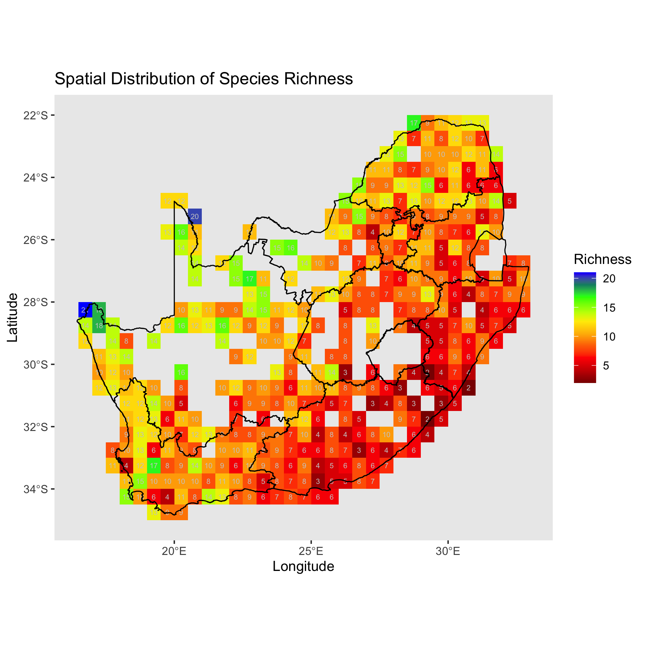
:chart_with_upwards_trend: Figure 4: Spatial distribution of species richness across the study area. Each grid cell shows the number of unique species (species richness) in each grid-cell.
:information_source: Why this matters: Early spatial diagnostics flag data gaps and uneven effort that can influence crowding and model fits.
:bulb: Summary: prepare_inputs() locks in a clean, aligned foundation for trait-based analyses; store fit and reference it throughout.
Generate hypothetical invaders:
Section titled “Generate hypothetical invaders: ”When invader traits are unknown, you can simulate plausible invaders from the resident pool to explore fitness scenarios. simulate_invaders() builds an invader trait table aligned with residents.
:hourglass_flowing_sand: What it does: It samples trait columns either independently (novel combinations) or row-wise (preserve covariance), supports bounded or distribution-based sampling for numerics, and honours factor levels.
:information_source: Why this matters: Simulation supports sensitivity analyses and planning when the exact invader set is uncertain.
:warning: Practical checks and tips: Prefer rowwise for realism when covariance is essential; use columnwise to probe unobserved combinations; keep trait names and levels identical to residents.
stopifnot(exists("simulate_invaders"))set.seed(42)
traits_inv = simulate_invaders(  resident_traits     = traits_res,  species_col         = NULL,  n_inv               = 10,  mode                = "columnwise",      # or "rowwise"  numeric_method      = "bootstrap",       # "tnorm" / "uniform"  keep_bounds         = TRUE,  inv_prefix          = "inv",  keep_species_column = TRUE,  seed                = 42)
traits_all = rbind(traits_res, traits_inv)head(traits_all[1:4,1:4]); tail(traits_all[1:4,1:4])#>                          trait_cont1 trait_cont2 trait_cont3 trait_cont4#> Acraea horta               0.8296121   0.8114763  -0.9221270  -0.6841896#> Amata cerbera              0.8741508  -0.1060607   0.4975908  -0.2819434#> Bicyclus safitza safitza  -0.4277209   0.6720085   0.3545537   0.2912638#> Cacyreus lingeus           0.6608953   0.4751912  -0.6574713   0.5516467#>                          trait_cont1 trait_cont2 trait_cont3 trait_cont4#> Acraea horta               0.8296121   0.8114763  -0.9221270  -0.6841896#> Amata cerbera              0.8741508  -0.1060607   0.4975908  -0.2819434#> Bicyclus safitza safitza  -0.4277209   0.6720085   0.3545537   0.2912638#> Cacyreus lingeus           0.6608953   0.4751912  -0.6574713   0.5516467
cat("Simulated invaders:", nrow(traits_inv),    "| invader traits:", ncol(traits_inv),    "| total species:", nrow(traits_all),    "| total traits:", ncol(traits_all), "\n")#> Simulated invaders: 10 | invader traits: 20 | total species: 37 | total traits: 20
:sparkles: Overall importance: This closes the data layer: residents, environment, and invaders are harmonised and ready for trait-space construction.
Shared trait space and resident crowding
Section titled “Shared trait space and resident crowding”This wrapper, prepare_trait_space(), builds the joint trait geometry (PCoA on Gower), diagnoses centrality and convex hull membership, and computes resident crowding
:hourglass_flowing_sand: What the wrapper does (step-by-step):
- Standardises traits leakage-safely;
- Computes Gower distances and PCoA scores;
- Identifies centroid, density, and hull;
- Builds
from Hellinger weights and Gaussian trait kernels; - Packages tidy diagnostics and plots.
Standardise model inputs (optional)
Section titled “Standardise model inputs (optional)”standardise_model_inputs() harmonises resident and invader traits and any numeric environment columns while preventing information leakage.
:hourglass_flowing_sand: Step-by-step: It z-scores resident traits and environment with a zero-variance guard ➔ scales invader numerics using resident moments ➔ coerces factor levels to resident sets ➔ optionally drops invader-only columns.
:information_source: Why this matters: Comparable scales improve ordination stability and GLMM convergence; resident-based scaling avoids leaking invader information.
:warning: Practical checks and tips: Keep invader columns a subset/compatible superset of residents; document factor level harmonisation.
Compute and plot the shared trait space
Section titled “Compute and plot the shared trait space”compute_trait_space() builds the unified trait map across residents and invaders using Gower dissimilarities followed by PCoA.
:hourglass_flowing_sand: Step-by-step: It computes distances across mixed types ➔ projects points to
:information_source: Why this matters: Positions relative to the hull and core foreshadow niche overlap and novelty, guiding the interpretation of crowding and abiotic alignment.
:warning: Practical checks and tips: Ensure >=3 residents for a stable hull; keep trait schemas identical; record ordination settings for reproducibility.
Determine centrality and convex-hull membership
Section titled “Determine centrality and convex-hull membership”compute_centrality_hull() quantifies where species sit relative to the resident cloud and whether invaders fall inside or outside the realised trait boundary.
:hourglass_flowing_sand: Step-by-step: It estimates robust covariance ➔ computes Mahalanobis distances ➔ rescales to centrality (0 = peripheral, 1 = core) ➔ and tests hull membership for each invader.
:information_source: Why this matters: Central or in-hull invaders face stronger crowding; peripheral or out-of-hull invaders may experience weaker biotic resistance if the environment suits.
:warning: Practical checks and tips: Use robust covariance to limit outlier leverage; keep a tidy table of ranks and flags for later map legends.
Resident crowding
Section titled “Resident crowding from composition × trait similarity”compute_resident_crowding() integrates community composition and trait similarity into site × resident crowding fields with optional per-site z-scores.
:hourglass_flowing_sand: Step-by-step: It Hellinger-transforms abundances to weights
:information_source: Why this matters:
:warning: Practical checks and tips: Verify name alignment between community and traits; examine distance distributions before fixing
:zap: Run prepare_trait_space() to construct the trait space, diagnostics, and fit.
stopifnot(inherits(fit, "invasimapr_fit"),          !is.null(fit$inputs$traits_res),          !is.null(fit$inputs$comm_res),          !is.null(fit$inputs$site_df))stopifnot(exists("traits_inv"))
# try(source("D:/Methods/R/myR_Packages/b-cubed-versions/invasimapr/R/prepare_trait_space.R"), silent = TRUE)# if (!exists("prepare_trait_space")) stop("prepare_trait_space() not found.")
fit = prepare_trait_space(  fit            = fit,  traits_inv     = traits_inv,  crowding_sigma = NULL,   # data-driven default  do_standardise = TRUE,  row_z          = FALSE,  show_plots     = FALSE)
# print(fit)# str(fit, 1)str(fit$traits, 1)#> List of 10#>  $ gower     : 'dissimilarity' Named num [1:666] 0.56 0.36 0.424 0.304 0.358 ...#>   ..- attr(*, "Labels")= chr [1:37] "Acraea horta" "Amata cerbera" "Bicyclus safitza safitza" "Cacyreus lingeus" ...#>   ..- attr(*, "Size")= int 37#>   ..- attr(*, "Metric")= chr "mixed"#>   ..- attr(*, "Types")= chr [1:20] "I" "I" "I" "I" ...#>  $ Q_res     :'data.frame':  27 obs. of  2 variables:#>  $ Q_inv     :'data.frame':  10 obs. of  2 variables:#>  $ hull      :'data.frame':  11 obs. of  2 variables:#>  $ centroid  : Named num [1:2] -4.88e-18 -2.25e-18#>   ..- attr(*, "names")= chr [1:2] "tr1" "tr2"#>  $ density   :List of 3#>  $ plots_ts  :List of 2#>  $ centrality: tibble [37 × 8] (S3: tbl_df/tbl/data.frame)#>  $ hull_df   :'data.frame':  11 obs. of  2 variables:#>  $ plots_ch  :List of 3str(fit$crowding, 1)#> List of 5#>  $ W_site     : num [1:415, 1:27] 0 0 0 0.238 0 ...#>   ..- attr(*, "dimnames")=List of 2#>   ..- attr(*, "parameters")=List of 2#>   ..- attr(*, "decostand")= chr "hellinger"#>  $ D_res      : num [1:27, 1:27] 0 0.56 0.36 0.424 0.304 ...#>   ..- attr(*, "dimnames")=List of 2#>  $ sigma_alpha: num 0.463#>  $ K_res_res  : num [1:27, 1:27] 0 0.482 0.739 0.658 0.806 ...#>   ..- attr(*, "dimnames")=List of 2#>  $ C_js       : num [1:415, 1:27] 2.14 1.63 1.84 2.21 1.88 ...#>   ..- attr(*, "dimnames")=List of 2
:card_index_dividers: Save the core trait geometry objects and crowding matrices used by the residents model and for invader predictions.
# Trait space & diagnosticsQ_res      = fit$traits$Q_resQ_inv      = fit$traits$Q_invgower_all  = fit$traits$gowerhull_res   = fit$traits$hullcentroid   = fit$traits$centroidcentral_df = fit$traits$centrality
# Resident crowdingC_js        = fit$crowding$C_jsC_js_z      = fit$crowding$C_js_zC_mu_s      = fit$crowding$C_mu_sC_sd_s      = fit$crowding$C_sd_sW_site      = fit$crowding$W_siteD_res       = fit$crowding$D_resK_res_res   = fit$crowding$K_res_ressigma_alpha = fit$crowding$sigma_alpha
# If standardisation rantraits_res_glmm = fit$inputs_std$traits_res_glmmtraits_inv_glmm = fit$inputs_std$traits_inv_glmm
Visualise different plots showing how invaders differ markedly in how much they overlap with resident trait strategies: For example, core invaders are more constrained by resident crowding, while peripheral invaders may exploit unfilled regions of trait space, though often at the cost of reduced environmental alignment. This framework links geometric novelty to invasion fitness expectations.
# Check output structure# str(fit$traits, 1)
# Heatmap plot# fit$traits$plots_ts$dens_plotfit$traits$plots_ts$dens_plot()  # draws to any current device (screen or file)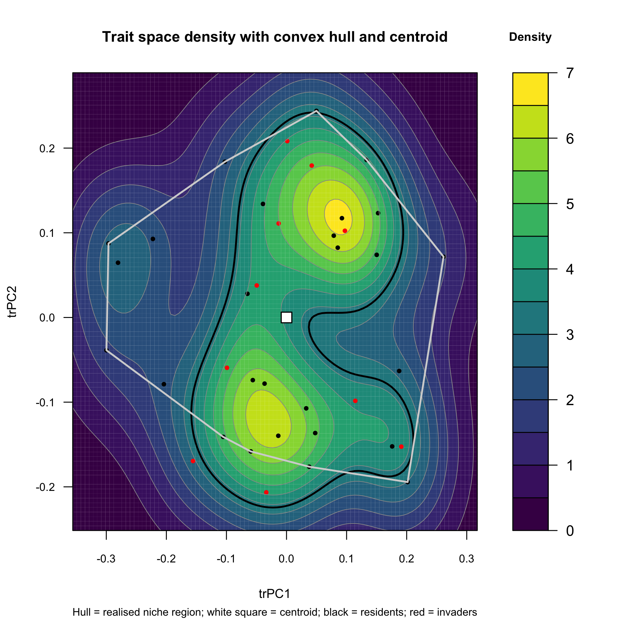
:chart_with_upwards_trend: Figure 5: Heatmap plot showing how all species are mapped into a shared trait space (PCoA on Gower distances). Coloured contours show kernel-density “hotspots” of resident strategies, the white polygon is the resident convex hull (realised niche region), and the white square marks the cloud centroid. Residents (black points) form a clearly multimodal structure with two dense modes (upper-right and lower-centre), separated by a lower-density corridor. Invaders (red points) are mostly inside the hull and often fall near the dense resident cores, positions that imply strong niche crowding penalties. A few invaders sit near the hull boundary or in sparser regions of trait space, indicating greater novelty and potentially weaker crowding if local abiotic suitability is high.
# Dendogram plotfit$traits$plots_ts$dend_plot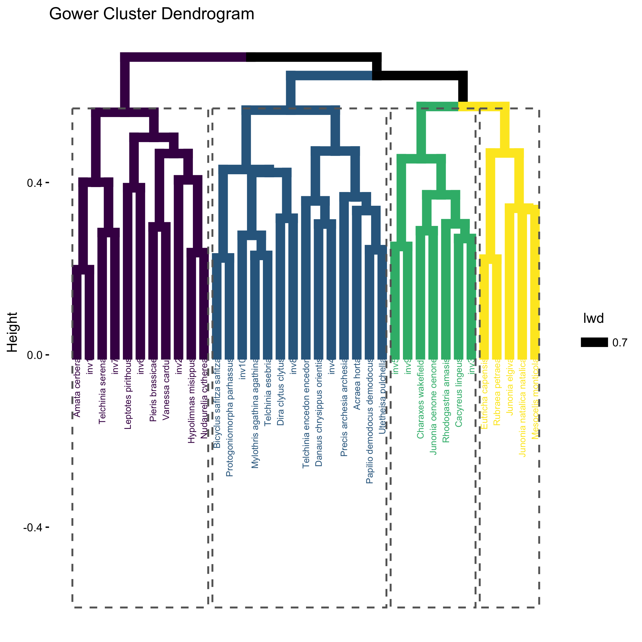
:chart_with_upwards_trend: Figure 6: Dendogram plot shows hierarchical clustering species using Gower distances. The large splits (branch heights) and coloured/dashed groups reveal distinct functional syndromes that align with the density modes in the trait map: a leftmost (purple) clade is well separated, while central clades (blue/green) encompass the dense core, and smaller rightmost clades (yellow) capture peripheral strategies. Together, the panels show a resident community with strong trait structure; invaders overlapping core clusters should experience higher
(crowding), whereas those on the periphery or near gaps in the hull may face weaker biotic resistance and thus higher establishment potential if is favourable.
:bar_chart: Centrality ranks and hull maps to highlight novelty and diagnose ordination and kernel choices. The three figures below, illustrate how invaders position relative to residents in trait space, and how this affects their potential to establish.
# Check output structure# str(fit$traits,1)# str(fit$traits$plots_ch, 1)# head(fit$crowding$C_js[1:4,1:4])
# Plot Centrality and hull statusif (!is.null(fit$traits$plots_ch)) {  print(fit$traits$plots_ch$p_trait)}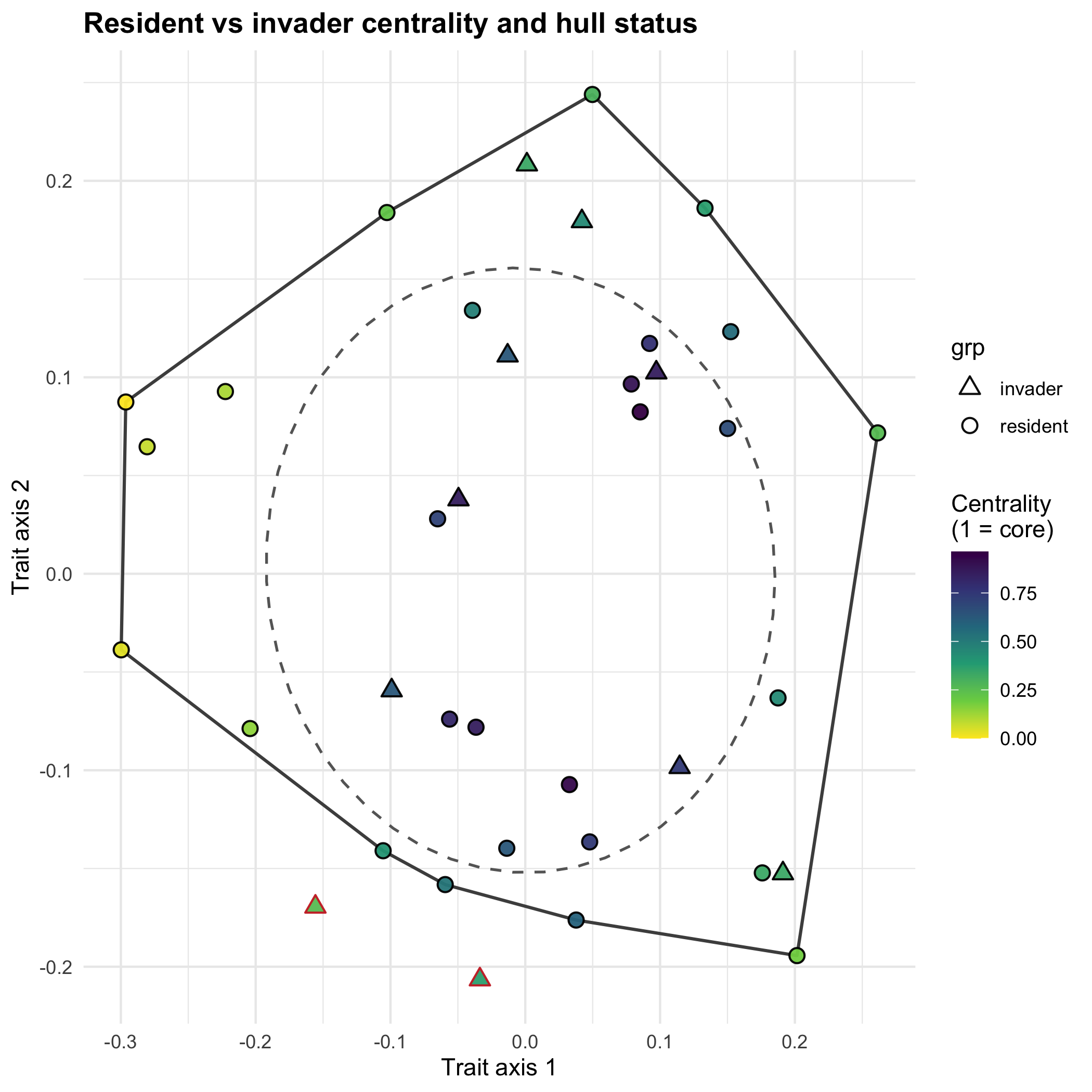
:chart_with_upwards_trend: Figure 7: Centrality and hull status shows residents (circles) and invaders (triangles) embedded in a two-dimensional trait space. The convex hull (solid polygon) marks the realised resident niche, while the dashed ellipse indicates the central core region. Colour shading reflects centrality (values closer to 1 are deeper within the resident cloud). Many invaders fall inside the hull but with relatively low centrality, placing them nearer the trait-space periphery. A few invaders lie outside the hull, representing novel strategies not currently expressed by residents.
# Plot Mahalanobis distance distributionfit$traits$plots_ch$p_dist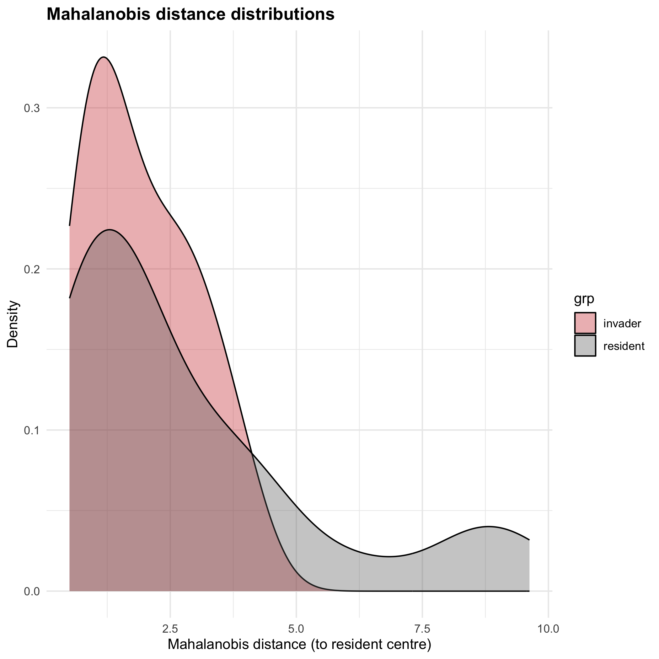
:chart_with_upwards_trend: Figure 8: Mahalanobis distance distribution comparisons from the resident centroid. Residents (grey) cluster close to the centre, with most distances below 2-3 units. Invaders (red) show a broader distribution, with some overlapping resident values but others displaced further into the tails. This highlights greater heterogeneity among invaders, with several occupying marginal or novel positions.
# Plot Invader ranking by centralityfit$traits$plots_ch$p_rank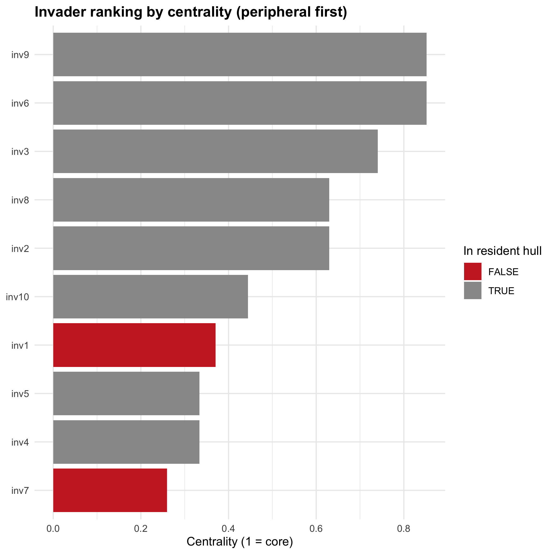
:chart_with_upwards_trend: Figure 9: Invader ranking by centrality (from peripheral to core). Peripheral invaders (low centrality) are often those falling outside the hull (red bars). These species represent the most novel introductions and are expected to experience weaker crowding, though their establishment will depend on abiotic suitability. Invaders with higher centrality (grey bars) overlap strongly with residents, implying greater competition and reduced establishment potential.
:sparkles: Overall importance: This stage anchors the trait geometry and the resident-side crowding fields that everything else builds on.
:bulb: Summary. You now have a reproducible trait map, novelty diagnostics, and
Resident predictors (standardised):
Section titled “Resident predictors (standardised): ”model_residents() fits a residents-only GLMM that yields site-standardised abiotic suitability
:hourglass_flowing_sand: What the wrapper does (step-by-step):
- Standardises environment and resident traits for the GLMM,
- Builds a transparent formula (with optional
interactions), - Fits
glmmTMB, - Predicts fixed-effects η for residents, and
- Applies per-site z-scores to
. - Computes
via a chosen mode and returns .
Build the model frame and formula
Section titled “Build the model frame and formula”build_model_formula() discovers predictors and assembles a formula that is reused for invaders to ensure consistent structure.
:hourglass_flowing_sand: Step-by-step: It infers environment and trait terms ➔ adds mains and optional (1|site) + (1|species) and optional zero-correlation random slopes ➔ returns a valid formula.
:information_source: Why this matters: Consistent specification across residents and invaders avoids scale drift and makes coefficients interpretable in the trait plane.
:warning: Checks/tips: Keep naming conventions stable (env_*, trait_*); avoid random slopes for site-only indices.
Fit the residents model (e.g., GLMM)
Section titled “Fit the residents model (e.g., GLMM)”prep_resident_glmm() expands the long site×resident frame, fits glmmTMB, and returns fixed-effect predictions as a site×resident matrix.
:hourglass_flowing_sand: Step-by-step: It joins site environment and resident traits ➔ coerces keys to factors ➔ fits a Tweedie log-link GLMM ➔ and predicts η with re.form = NA.
:information_source: Why this matters: Fixed-effect predictions provide an abiotic suitability surface without borrowing random effects across species or sites.
:warning: Checks/tips: Ensure numeric matrices, no NA predictors, and sensible convergence (simplify interactions if needed).
Site-standardised resident predictors
Section titled “Site-standardised resident predictors”standardise_by_site() centres and scales each site row for
:hourglass_flowing_sand: Step-by-step: It computes row means and SDs (robust optional) ➔ guards zero SD ➔ and returns z-scores plus moments.
:information_source: Why this matters: Within-site scaling makes predictors comparable across species and ensures invaders can be standardised on resident moments.
:warning: Checks/tips: Prefer robust scaling for skewed row_mean and row_sd for invader standardisation.
Site-only saturation
Section titled “Site-only saturation and global z-score”compute_site_saturation() builds a site-only competition index from totals, modelled dominance, or evenness deficit, then applies a global z-score and broadcasts to species.
:hourglass_flowing_sand: Step-by-step: It computes S_js_z for residents.
:information_source: Why this matters:
:warning: Checks/tips: Do not add random slopes on
:zap: Run model_residents() to fit the resident model (e.g. GLMM), construct standardised predictors, and write results back to fit$model and fit$residents.
# try(source("D:/Methods/R/myR_Packages/b-cubed-versions/invasimapr/R/model_residents.R"), silent = TRUE)# if (!exists("model_residents")) stop("model_residents() not found.")
# Run model_residents() functionfit = model_residents(  fit,  family = glmmTMB::tweedie(link = "log"),  include_env_trait_interactions = TRUE,  saturation_mode = "evenness_deficit",  reduce_strategy = 'none',  robust_r = TRUE)
# print(fit)# str(fit$model, 1)# str(fit$residents, 1)summary(fit$residents$fit_r)#>  Family: tweedie  ( log )#> Formula:          abundance ~ env1 + env2 + env3 + env4 + env5 + env6 + env7 +#>     env8 + env9 + env10 + trait_cont1 + trait_cont2 + trait_cont3 +#>     trait_cont4 + trait_cont5 + trait_cont6 + trait_cont7 + trait_cont8 +#>     trait_cont9 + trait_cont10 + trait_cat11 + trait_cat12 +#>     trait_cat13 + trait_cat14 + trait_cat15 + trait_ord16 + trait_ord17 +#>     trait_bin18 + trait_bin19 + trait_ord20 + (env1 + env2 +#>     env3 + env4 + env5 + env6 + env7 + env8 + env9 + env10):(trait_cont1 +#>     trait_cont2 + trait_cont3 + trait_cont4 + trait_cont5 + trait_cont6 +#>     trait_cont7 + trait_cont8 + trait_cont9 + trait_cont10 +#>     trait_cat11 + trait_cat12 + trait_cat13 + trait_cat14 + trait_cat15 +#>     trait_ord16 + trait_ord17 + trait_bin18 + trait_bin19 + trait_ord20) +#>     (1 | site) + (1 | species)#> Data: attempt$rg$dat_r#>#>       AIC       BIC    logLik -2*log(L)  df.resid#>   38197.5   40241.0  -18819.8   37639.5     10926#>#> Random effects:#>#> Conditional model:#>  Groups  Name        Variance Std.Dev.#>  site    (Intercept) 0.006301 0.07938#>  species (Intercept) 0.001645 0.04056#> Number of obs: 11205, groups:  site, 415; species, 27#>#> Dispersion parameter for tweedie family (): 7.98#>#> Conditional model:#>                                 Estimate Std. Error z value Pr(>|z|)#> (Intercept)                    1.2833901  0.1361082   9.429  < 2e-16 ***#> env1                           0.4238189  0.2730032   1.552 0.120559#> env2                          -0.4629570  0.2814522  -1.645 0.099993 .#> env3                          -0.1523661  0.3976060  -0.383 0.701565#> env4                           0.2574086  0.3011752   0.855 0.392728#> env5                           0.2883784  0.3298333   0.874 0.381946#> env6                           0.0920454  0.3380372   0.272 0.785396#> env7                           0.1802530  0.4869892   0.370 0.711280#> env8                          -0.1178539  0.4933806  -0.239 0.811206#> env9                          -0.1477103  0.4607070  -0.321 0.748501#> env10                         -0.2388646  0.5557325  -0.430 0.667327#> trait_cont1                   -0.2879529  0.0995748  -2.892 0.003830 **#> trait_cont2                   -0.1468610  0.0429340  -3.421 0.000625 ***#> trait_cont3                   -0.0183904  0.0671736  -0.274 0.784258#> trait_cont4                    0.0057871  0.0526189   0.110 0.912425#> trait_cont5                    0.0329278  0.0538160   0.612 0.540631#> trait_cont6                    0.0446251  0.0734411   0.608 0.543432#> trait_cont7                   -0.0332561  0.0488246  -0.681 0.495787#> trait_cont8                    0.0582392  0.0701413   0.830 0.406362#> trait_cont9                   -0.0030572  0.0521304  -0.059 0.953235#> trait_cont10                   0.0757443  0.0495473   1.529 0.126332#> trait_cat11grassland           0.0384514  0.1842370   0.209 0.834678#> trait_cat11wetland            -0.1194091  0.2430696  -0.491 0.623246#> trait_cat12nocturnal          -0.2214629  0.1160278  -1.909 0.056300 .#> trait_cat13multivoltine        0.0069169  0.0965116   0.072 0.942866#> trait_cat13univoltine         -0.1972040  0.1309296  -1.506 0.132020#> trait_cat14generalist          0.0380147  0.2600996   0.146 0.883799#> trait_cat14nectarivore         0.2441572  0.1720548   1.419 0.155880#> trait_cat15resident           -0.0448762  0.1352528  -0.332 0.740044#> trait_ord16                    0.0155845  0.0581019   0.268 0.788525#> trait_ord17                   -0.0457999  0.0426140  -1.075 0.282481#> trait_bin18                    0.0384106  0.0484466   0.793 0.427869#> trait_bin19                    0.0104646  0.0576802   0.181 0.856035#> trait_ord20medium              0.0838120  0.2635444   0.318 0.750471#> trait_ord20small              -0.1652942  0.1540706  -1.073 0.283340#> env1:trait_cont1               0.2590543  0.2018959   1.283 0.199454#> env1:trait_cont2               0.0511837  0.0872490   0.587 0.557446#> env1:trait_cont3               0.0419782  0.1365365   0.307 0.758500#> env1:trait_cont4               0.0569235  0.1068453   0.533 0.594196#> env1:trait_cont5              -0.1396320  0.1099753  -1.270 0.204203#> env1:trait_cont6              -0.1149766  0.1490549  -0.771 0.440487#> env1:trait_cont7               0.0247308  0.1007236   0.246 0.806045#> env1:trait_cont8              -0.0832165  0.1424527  -0.584 0.559107#> env1:trait_cont9               0.0193295  0.1069047   0.181 0.856516#> env1:trait_cont10             -0.0166879  0.1012074  -0.165 0.869032#> env1:trait_cat11grassland     -0.2495010  0.3716669  -0.671 0.502028#> env1:trait_cat11wetland       -0.2737927  0.4937667  -0.554 0.579238#> env1:trait_cat12nocturnal     -0.0896390  0.2365215  -0.379 0.704696#> env1:trait_cat13multivoltine   0.1300371  0.1954317   0.665 0.505805#> env1:trait_cat13univoltine     0.2479814  0.2637601   0.940 0.347126#> env1:trait_cat14generalist     0.1803710  0.5286677   0.341 0.732968#> env1:trait_cat14nectarivore   -0.2256056  0.3489209  -0.647 0.517903#> env1:trait_cat15resident      -0.1195242  0.2759828  -0.433 0.664952#> env1:trait_ord16               0.0164264  0.1176699   0.140 0.888978#> env1:trait_ord17              -0.0983943  0.0860021  -1.144 0.252585#> env1:trait_bin18              -0.0447998  0.0978090  -0.458 0.646928#> env1:trait_bin19              -0.0989036  0.1160240  -0.852 0.393970#> env1:trait_ord20medium        -0.1203885  0.5353213  -0.225 0.822065#> env1:trait_ord20small          0.2076244  0.3127982   0.664 0.506841#> env2:trait_cont1              -0.1073236  0.2099272  -0.511 0.609182#> env2:trait_cont2               0.0998720  0.0909106   1.099 0.271954#> env2:trait_cont3              -0.0302382  0.1432439  -0.211 0.832812#> env2:trait_cont4               0.0062584  0.1123871   0.056 0.955592#> env2:trait_cont5              -0.0215891  0.1145595  -0.188 0.850522#> env2:trait_cont6               0.0958735  0.1549708   0.619 0.536143#> env2:trait_cont7              -0.1614124  0.1051725  -1.535 0.124848#> env2:trait_cont8              -0.1579836  0.1475678  -1.071 0.284357#> env2:trait_cont9              -0.0824353  0.1116071  -0.739 0.460137#> env2:trait_cont10              0.0042922  0.1059621   0.041 0.967689#> env2:trait_cat11grassland      0.3465967  0.3880252   0.893 0.371733#> env2:trait_cat11wetland       -0.1429870  0.5138745  -0.278 0.780818#> env2:trait_cat12nocturnal     -0.0109025  0.2464091  -0.044 0.964709#> env2:trait_cat13multivoltine   0.0772089  0.2022998   0.382 0.702717#> env2:trait_cat13univoltine    -0.0152930  0.2723597  -0.056 0.955222#> env2:trait_cat14generalist     0.0938038  0.5469770   0.171 0.863835#> env2:trait_cat14nectarivore    0.0034584  0.3626978   0.010 0.992392#> env2:trait_cat15resident       0.0934440  0.2852982   0.328 0.743266#> env2:trait_ord16               0.1898966  0.1219071   1.558 0.119301#> env2:trait_ord17               0.1206038  0.0899711   1.340 0.180092#> env2:trait_bin18               0.0037917  0.1020570   0.037 0.970363#> env2:trait_bin19               0.0436744  0.1229657   0.355 0.722458#> env2:trait_ord20medium        -0.1337030  0.5551158  -0.241 0.809667#> env2:trait_ord20small          0.1591382  0.3209528   0.496 0.620014#> env3:trait_cont1              -0.0372629  0.2951912  -0.126 0.899548#> env3:trait_cont2               0.0420001  0.1284998   0.327 0.743782#> env3:trait_cont3               0.0621160  0.1991385   0.312 0.755099#> env3:trait_cont4               0.0263516  0.1563270   0.169 0.866137#> env3:trait_cont5              -0.0431644  0.1605220  -0.269 0.788006#> env3:trait_cont6               0.1030986  0.2177213   0.474 0.635832#> env3:trait_cont7              -0.1336400  0.1481034  -0.902 0.366875#> env3:trait_cont8              -0.0871097  0.2080141  -0.419 0.675385#> env3:trait_cont9               0.0312030  0.1557542   0.200 0.841219#> env3:trait_cont10             -0.0836775  0.1486914  -0.563 0.573599#> env3:trait_cat11grassland      0.0530339  0.5416079   0.098 0.921996#> env3:trait_cat11wetland        0.0004273  0.7215614   0.001 0.999527#> env3:trait_cat12nocturnal      0.0338567  0.3435294   0.099 0.921491#> env3:trait_cat13multivoltine  -0.0355021  0.2866598  -0.124 0.901436#> env3:trait_cat13univoltine    -0.0267714  0.3821760  -0.070 0.944154#> env3:trait_cat14generalist    -0.0064808  0.7741574  -0.008 0.993321#> env3:trait_cat14nectarivore    0.1040584  0.5059753   0.206 0.837057#> env3:trait_cat15resident       0.1061745  0.4041305   0.263 0.792764#> env3:trait_ord16               0.0159803  0.1718122   0.093 0.925895#> env3:trait_ord17               0.1282873  0.1257695   1.020 0.307719#> env3:trait_bin18              -0.1023514  0.1429024  -0.716 0.473848#> env3:trait_bin19               0.0989221  0.1715115   0.577 0.564097#> env3:trait_ord20medium        -0.0583839  0.7834286  -0.075 0.940594#> env3:trait_ord20small          0.0076437  0.4583593   0.017 0.986695#> env4:trait_cont1               0.1871081  0.2217728   0.844 0.398841#> env4:trait_cont2              -0.0448973  0.0951791  -0.472 0.637131#> env4:trait_cont3               0.1660386  0.1507123   1.102 0.270595#> env4:trait_cont4               0.0513924  0.1184007   0.434 0.664248#> env4:trait_cont5               0.0259057  0.1226941   0.211 0.832777#> env4:trait_cont6              -0.0927677  0.1635505  -0.567 0.570570#> env4:trait_cont7               0.1163699  0.1121210   1.038 0.299319#> env4:trait_cont8              -0.0180249  0.1561764  -0.115 0.908117#> env4:trait_cont9               0.0772283  0.1170715   0.660 0.509467#> env4:trait_cont10             -0.0208430  0.1107179  -0.188 0.850678#> env4:trait_cat11grassland     -0.1799181  0.4028088  -0.447 0.655122#> env4:trait_cat11wetland        0.3953166  0.5415347   0.730 0.465394#> env4:trait_cat12nocturnal     -0.0130807  0.2587156  -0.051 0.959676#> env4:trait_cat13multivoltine  -0.0585961  0.2173298  -0.270 0.787454#> env4:trait_cat13univoltine     0.0947713  0.2903156   0.326 0.744090#> env4:trait_cat14generalist     0.0786553  0.5813832   0.135 0.892383#> env4:trait_cat14nectarivore    0.0233595  0.3815324   0.061 0.951180#> env4:trait_cat15resident      -0.1226286  0.3045990  -0.403 0.687250#> env4:trait_ord16              -0.1742459  0.1306910  -1.333 0.182444#> env4:trait_ord17              -0.0095848  0.0936071  -0.102 0.918444#> env4:trait_bin18               0.1460148  0.1070335   1.364 0.172505#> env4:trait_bin19              -0.1382084  0.1268928  -1.089 0.276077#> env4:trait_ord20medium        -0.1994732  0.5888167  -0.339 0.734783#> env4:trait_ord20small         -0.2580449  0.3457473  -0.746 0.455462#> env5:trait_cont1               0.0123702  0.2456663   0.050 0.959841#> env5:trait_cont2              -0.0609928  0.1066625  -0.572 0.567438#> env5:trait_cont3               0.0756810  0.1652044   0.458 0.646877#> env5:trait_cont4               0.0216662  0.1288836   0.168 0.866499#> env5:trait_cont5               0.0346696  0.1318799   0.263 0.792637#> env5:trait_cont6              -0.0602581  0.1811538  -0.333 0.739410#> env5:trait_cont7               0.0551824  0.1224985   0.450 0.652368#> env5:trait_cont8               0.0679692  0.1728442   0.393 0.694142#> env5:trait_cont9               0.0678823  0.1291918   0.525 0.599278#> env5:trait_cont10             -0.0582309  0.1233393  -0.472 0.636841#> env5:trait_cat11grassland     -0.1218774  0.4491573  -0.271 0.786124#> env5:trait_cat11wetland        0.0071179  0.6004955   0.012 0.990543#> env5:trait_cat12nocturnal     -0.1119143  0.2868002  -0.390 0.696376#> env5:trait_cat13multivoltine  -0.1107300  0.2358441  -0.470 0.638709#> env5:trait_cat13univoltine    -0.2036733  0.3176916  -0.641 0.521455#> env5:trait_cat14generalist    -0.2461068  0.6403223  -0.384 0.700720#> env5:trait_cat14nectarivore   -0.0526845  0.4223282  -0.125 0.900723#> env5:trait_cat15resident       0.0484835  0.3353476   0.145 0.885045#> env5:trait_ord16              -0.0811707  0.1411523  -0.575 0.565252#> env5:trait_ord17              -0.0972289  0.1035414  -0.939 0.347713#> env5:trait_bin18               0.1027040  0.1188081   0.864 0.387339#> env5:trait_bin19              -0.0636271  0.1419014  -0.448 0.653872#> env5:trait_ord20medium         0.0120206  0.6490946   0.019 0.985225#> env5:trait_ord20small         -0.2150638  0.3789890  -0.567 0.570397#> env6:trait_cont1              -0.0246898  0.2480779  -0.100 0.920722#> env6:trait_cont2              -0.0004339  0.1071391  -0.004 0.996769#> env6:trait_cont3               0.0226814  0.1673397   0.136 0.892184#> env6:trait_cont4               0.0534481  0.1317414   0.406 0.684960#> env6:trait_cont5               0.1094548  0.1359880   0.805 0.420886#> env6:trait_cont6               0.1142859  0.1832831   0.624 0.532924#> env6:trait_cont7               0.1214664  0.1249329   0.972 0.330925#> env6:trait_cont8               0.1004448  0.1755440   0.572 0.567192#> env6:trait_cont9               0.0738422  0.1303336   0.567 0.571011#> env6:trait_cont10              0.0337164  0.1243256   0.271 0.786241#> env6:trait_cat11grassland     -0.3415737  0.4513362  -0.757 0.449166#> env6:trait_cat11wetland       -0.1465829  0.6027141  -0.243 0.807847#> env6:trait_cat12nocturnal      0.2060312  0.2883638   0.714 0.474928#> env6:trait_cat13multivoltine  -0.2666277  0.2412991  -1.105 0.269174#> env6:trait_cat13univoltine     0.2117171  0.3250485   0.651 0.514827#> env6:trait_cat14generalist    -0.3044428  0.6501297  -0.468 0.639584#> env6:trait_cat14nectarivore   -0.0652948  0.4260207  -0.153 0.878188#> env6:trait_cat15resident       0.0024190  0.3407272   0.007 0.994335#> env6:trait_ord16              -0.1436754  0.1453234  -0.989 0.322830#> env6:trait_ord17               0.0901250  0.1052978   0.856 0.392050#> env6:trait_bin18              -0.0602324  0.1202303  -0.501 0.616388#> env6:trait_bin19               0.0404023  0.1420808   0.284 0.776133#> env6:trait_ord20medium         0.3375212  0.6570004   0.514 0.607440#> env6:trait_ord20small          0.0095392  0.3848254   0.025 0.980224#> env7:trait_cont1              -0.1730178  0.3627418  -0.477 0.633382#> env7:trait_cont2              -0.0316228  0.1574463  -0.201 0.840817#> env7:trait_cont3              -0.1838059  0.2450052  -0.750 0.453127#> env7:trait_cont4               0.0300894  0.1917809   0.157 0.875328#> env7:trait_cont5              -0.1932804  0.1958736  -0.987 0.323760#> env7:trait_cont6              -0.0130956  0.2664564  -0.049 0.960802#> env7:trait_cont7              -0.0292479  0.1810542  -0.162 0.871666#> env7:trait_cont8               0.0192467  0.2547439   0.076 0.939775#> env7:trait_cont9               0.0404890  0.1916159   0.211 0.832651#> env7:trait_cont10              0.0584509  0.1818610   0.321 0.747904#> env7:trait_cat11grassland     -0.1630086  0.6679496  -0.244 0.807197#> env7:trait_cat11wetland        0.0845999  0.8871659   0.095 0.924029#> env7:trait_cat12nocturnal     -0.3929308  0.4254169  -0.924 0.355675#> env7:trait_cat13multivoltine  -0.0399157  0.3498784  -0.114 0.909171#> env7:trait_cat13univoltine     0.0647597  0.4663271   0.139 0.889551#> env7:trait_cat14generalist     0.2251639  0.9501766   0.237 0.812680#> env7:trait_cat14nectarivore    0.1571325  0.6249955   0.251 0.801494#> env7:trait_cat15resident      -0.1963711  0.4947895  -0.397 0.691457#> env7:trait_ord16               0.0412175  0.2100704   0.196 0.844447#> env7:trait_ord17              -0.1892053  0.1544197  -1.225 0.220475#> env7:trait_bin18              -0.0525759  0.1748677  -0.301 0.763673#>  [ reached 'max' / getOption("max.print") -- omitted 75 rows ]#> ---#> Signif. codes:  0 '***' 0.001 '**' 0.01 '*' 0.05 '.' 0.1 ' ' 1
:card_index_dividers: Save the core resident model objects used for invader predictions.
str(fit$residents, 1)#> List of 16#>  $ fit_r   :List of 7#>   ..- attr(*, "class")= chr "glmmTMB"#>  $ dat_r   :'data.frame':  11205 obs. of  33 variables:#>  $ grid_res:'data.frame':  11205 obs. of  33 variables:#>  $ fml     :Class 'formula'  language abundance ~ env1 + env2 + env3 + env4 + env5 + env6 + env7 + env8 + env9 + env10 + trait_cont1 +      trait_cont2| __truncated__ ...#>   .. ..- attr(*, ".Environment")=<environment: 0x89207ccf0>#>  $ r_js    : num [1:415, 1:27] 1.061 0.957 1.218 1.247 1.415 ...#>   ..- attr(*, "dimnames")=List of 2#>  $ mu_js   : num [1:415, 1:27] 2.89 2.6 3.38 3.48 4.12 ...#>   ..- attr(*, "dimnames")=List of 2#>  $ r_js_z  : num [1:415, 1:27] -0.1157 -0.2056 0.0858 -0.1993 0.1854 ...#>   ..- attr(*, "dimnames")=List of 2#>  $ r_mu_s  : Named num [1:415] 1.17 1.14 1.14 1.39 1.25 ...#>   ..- attr(*, "names")= chr [1:415] "82" "83" "84" "117" ...#>  $ r_sd_s  : Named num [1:415] 0.906 0.909 0.884 0.703 0.898 ...#>   ..- attr(*, "names")= chr [1:415] "82" "83" "84" "117" ...#>  $ C_js_z  : num [1:415, 1:27] 1.028 -1.057 1.46 0.881 1.484 ...#>   ..- attr(*, "dimnames")=List of 2#>  $ C_mu_s  : Named num [1:415] 1.98 1.74 1.61 2.06 1.61 ...#>   ..- attr(*, "names")= chr [1:415] "82" "83" "84" "117" ...#>  $ C_sd_s  : Named num [1:415] 0.154 0.101 0.159 0.177 0.176 ...#>   ..- attr(*, "names")= chr [1:415] "82" "83" "84" "117" ...#>  $ S_s     : Named num [1:415] 0.0798 0.025 0.1327 0.1478 0.226 ...#>   ..- attr(*, "names")= chr [1:415] "82" "83" "84" "117" ...#>  $ S_s_z   : Named num [1:415] 0.172 -1.104 1.406 1.758 3.579 ...#>   ..- attr(*, "names")= chr [1:415] "82" "83" "84" "117" ...#>  $ S_js_z  : num [1:415, 1:27] 0.172 -1.104 1.406 1.758 3.579 ...#>   ..- attr(*, "dimnames")=List of 2#>  $ messages: chr [1:2] "preflight_gb=0.02" "path=original"r_js    = fit$residents$r_jsr_js_z  = fit$residents$r_js_zC_js_z  = fit$residents$C_js_zS_s_z   = fit$residents$S_s_zS_js_z  = fit$residents$S_js_z
r_mu_s  = fit$residents$r_mu_sr_sd_s  = fit$residents$r_sd_s
:bar_chart: Site map of
# str(fit$residents,1)head(fit$residents$S_js_z[1:4,1:4])#>     Acraea horta Amata cerbera Bicyclus safitza safitza Cacyreus lingeus#> 82     0.1720317     0.1720317                0.1720317        0.1720317#> 83    -1.1043100    -1.1043100               -1.1043100       -1.1043100#> 84     1.4055746     1.4055746                1.4055746        1.4055746#> 117    1.7579032     1.7579032                1.7579032        1.7579032
site_sat_df = data.frame(  site  = names(fit$residents$S_s_z),  S_s_z = as.numeric(fit$residents$S_s_z),  row.names = NULL, check.names = FALSE) |>  dplyr::left_join(site_df, by = "site")
ggplot2::ggplot(site_sat_df, ggplot2::aes(x, y, fill = S_s_z)) +  ggplot2::geom_tile() +  ggplot2::scale_fill_viridis_c(name=expression(Mean~S^{(z)}), direction=-1) +  ggplot2::geom_sf(data = rsa, inherit.aes = FALSE, fill = NA, color = "black", size = 0.3) +  ggplot2::labs(title = expression("Mean saturation (" * S^z * ") across sites"), x = "Longitude", y = "Latitude") +  ggplot2::theme_minimal()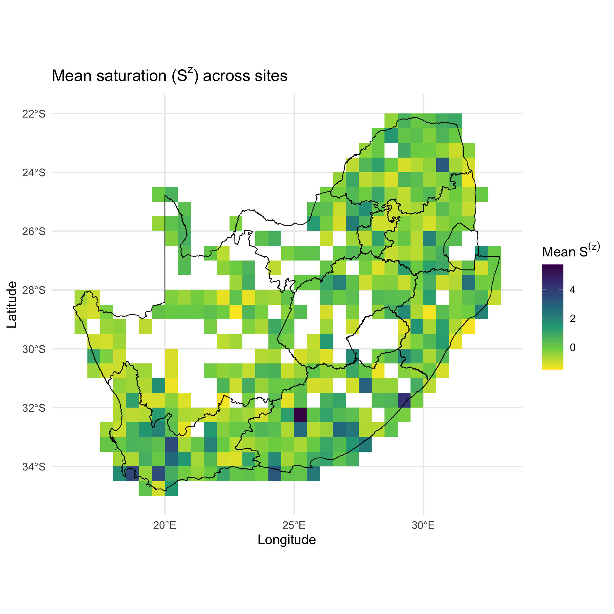
:chart_with_upwards_trend: Figures 10: The map shows the mean saturation term (
) across sites in South Africa, calculated from the relative abundance structure of resident communities. Warmer colours (yellow) indicate sites with low saturation values, suggesting lower levels of resident dominance, whereas cooler colours (green to purple) highlight sites with higher saturation, where resident communities are dense and strongly filled. The pattern is heterogeneous: several regions, including the south-western Cape and parts of the interior plateau, show pronounced hotspots of high saturation, while coastal and northern areas are more lightly saturated. This map is an important diagnostic for the site saturation predictor in the invasion fitness framework. Areas of high reflect environments where invaders are expected to experience stronger suppression from resident dominance, regardless of their trait alignment. Conversely, low-saturation sites highlight potential windows of opportunity where invaders may establish more easily if abiotic suitability and trait differences align.
:zap: In practice, visualising
:sparkles: Overall importance: This step produces resident-only, site-comparable predictors that define the scale on which invaders will be evaluated.
:bulb: Summary. You now have
Learn trait- and site-varying sensitivities (
Section titled “Learn trait- and site-varying sensitivities ()”learn_sensitivities() fits an auxiliary GLMM to relate
:hourglass_flowing_sand: What the wrapper does (step-by-step):
- Builds a long residents table with
, - Fits interactions between predictors and the trait plane,
- Extracts slopes to compute
, (signed optional), , - Applies a test for trait-varying
(Wald by default; likelihood-ratio test (LRT) optional), and - (optionally) Combines site random slopes to produce
and .
Auxiliary residents-only model on standardised predictors
Section titled “Auxiliary residents-only model on standardised predictors”fit_auxiliary_residents_glmm() estimates how slopes on
:hourglass_flowing_sand: Step-by-step: It creates one row per site × resident ➔ adds predictors and trait coordinates ➔ fits interactions (r_z + C_z + S_z) × (tr1 + tr2) with (1|site) + (1|species) and optional site random slopes for r_z and C_z.
:information_source: Why this matters: The fitted slope systems underpin trait-varying and site-varying sensitivities for invasion fitness.
:warning: Checks/tips: Ensure re.form = NA when predicting; avoid slopes on site-only S_z.
Trait-varying sensitivities and
Section titled “Trait-varying sensitivities and ”derive_sensitivities() parses fixed effects to compute trait-dependent coefficients and chooses
:hourglass_flowing_sand: Step-by-step: It evaluates slopes at each invader’s
:information_source: Why this matters: These parameters translate trait position into how hard crowding bites and how steep abiotic gains are.
:warning: Checks/tips: Match Q_inv rownames and columns; inspect distributions of lrt = "lrt" for a likelihood-ratio test, or lrt = "none" to skip testing.
Site-varying penalties and slopes
Section titled “Site-varying penalties and slopes and ”site_varying_alpha_beta_gamma() combines trait-varying slopes with site random-slope deviations to form site×invader versions where appropriate.
:hourglass_flowing_sand: Step-by-step: It sums fixed and random-slope parts for C_z and r_z ➔ clamps
:information_source: Why this matters: Site heterogeneity modulates how universal or local the inferred penalties and gains are.
:warning: Checks/tips: Include (0 + C_z || site) and optionally (0 + r_z || site) in the auxiliary model; weak random-slope variance implies little site variation.
:zap: Run learn_sensitivities() to fit the auxiliary model, derive trait- and site-varying sensitivities, and attach them to fit$sensitivities.
# try(source("D:/Methods/R/myR_Packages/b-cubed-versions/invasimapr/R/learn_sensitivities.R"), silent = TRUE)# if (!exists("learn_sensitivities")) stop("learn_sensitivities() not found.")
fit = learn_sensitivities(  fit,  use_site_random_slopes = TRUE,  lrt = TRUE)
str(fit$sensitivities, 1)#> List of 26#>  $ fit_coeffs           :List of 7#>   ..- attr(*, "class")= chr "glmmTMB"#>  $ data_used            : tibble [11,205 × 8] (S3: tbl_df/tbl/data.frame)#>  $ formula              :Class 'formula'  language log1p(abundance) ~ (r_z + C_z + S_z) * (tr1 + tr2) + (1 | species) + (1 | site) + (0 + r_z ||      site) + (0 + C_z || site)#>   .. ..- attr(*, ".Environment")=<environment: 0x89d569e70>#>  $ alpha_i              : Named num [1:10] 0.982 0.964 0.973 0.981 0.937 ...#>   ..- attr(*, "names")= chr [1:10] "inv1" "inv2" "inv3" "inv4" ...#>  $ alpha_signed_i       : Named num [1:10] 0.982 0.964 0.973 0.981 0.937 ...#>   ..- attr(*, "names")= chr [1:10] "inv1" "inv2" "inv3" "inv4" ...#>  $ beta_i               : Named num [1:10] 0.0883 0.0695 0.0833 0.0925 0.045 ...#>   ..- attr(*, "names")= chr [1:10] "inv1" "inv2" "inv3" "inv4" ...#>  $ beta_signed_i        : Named num [1:10] -0.0883 -0.0695 -0.0833 -0.0925 -0.045 ...#>   ..- attr(*, "names")= chr [1:10] "inv1" "inv2" "inv3" "inv4" ...#>  $ theta0               : num 0.213#>  $ theta_i              : Named num [1:10] 0.231 0.21 0.233 0.245 0.192 ...#>   ..- attr(*, "names")= chr [1:10] "inv1" "inv2" "inv3" "inv4" ...#>  $ gamma_i              : Named num [1:10] 0.213 0.213 0.213 0.213 0.213 ...#>   ..- attr(*, "names")= chr [1:10] "inv1" "inv2" "inv3" "inv4" ...#>  $ wald_lrt             :'data.frame':  1 obs. of  4 variables:#>  $ sens_df              :'data.frame':  10 obs. of  13 variables:#>  $ clamp_summary        :List of 5#>  $ prior_note           : chr "Biotic effects are modelled as nonnegative penalties; positive learned slopes are reported but not used to increase lambda."#>  $ site_alpha_beta_gamma:List of 12#>  $ alpha_is             : num [1:415, 1:10] 1.123 0.715 0.941 0.609 1.015 ...#>   ..- attr(*, "dimnames")=List of 2#>  $ Gamma_is             : num [1:415, 1:10] 0.33 -0.126 0.512 0.752 0.382 ...#>   ..- attr(*, "dimnames")=List of 2#>  $ site_alpha           :List of 4#>  $ site_gamma           :List of 4#>  $ a0                   : num -0.96#>  $ a1                   : num -0.0226#>  $ a2                   : num 0.11#>  $ b0                   : num -0.0675#>  $ b1                   : num -0.0447#>  $ b2                   : num 0.108#>  $ abg_df               :'data.frame':  4150 obs. of  12 variables:
alpha_i        = fit$sensitivities$alpha_ibeta_i         = fit$sensitivities$beta_ibeta_signed_i  = fit$sensitivities$beta_signed_itheta0         = fit$sensitivities$theta0theta_i        = fit$sensitivities$theta_igamma_i        = fit$sensitivities$gamma_ialpha_is       = fit$sensitivities$alpha_isGamma_is       = fit$sensitivities$Gamma_issens_df        = fit$sensitivities$sens_dfabg_df         = fit$sensitivities$abg_df
head(sens_df[1:4,1:4]); head(abg_df[1:4,1:4])#>   invader         tr1         tr2  slope_C_i#> 1    inv1 -0.03366963 -0.20651611 -0.9815948#> 2    inv2 -0.09911835 -0.05940586 -0.9639289#> 3    inv3  0.11449719 -0.09846095 -0.9730468#> 4    inv4  0.19113440 -0.15252673 -0.9807258#>   site invader  alpha_is SLOPE_C_is#> 1   82    inv1 1.1226958 -1.1226958#> 2   83    inv1 0.7148899 -0.7148899#> 3   84    inv1 0.9412440 -0.9412440#> 4  117    inv1 0.6092374 -0.6092374
:bar_chart: Heatmaps of
ggplot2::ggplot(abg_df, ggplot2::aes(invader, site, fill = alpha_is)) + ggplot2::geom_tile() + ggplot2::scale_fill_viridis_c(name = expression(alpha[is])) + ggplot2::labs(title = expression("Site-varying " * alpha[is]), x = "Invader", y = "Site") + ggplot2::theme_minimal(base_size = 11) + ggplot2::theme(axis.text.x = ggplot2::element_text(angle = 90, vjust = 0.5))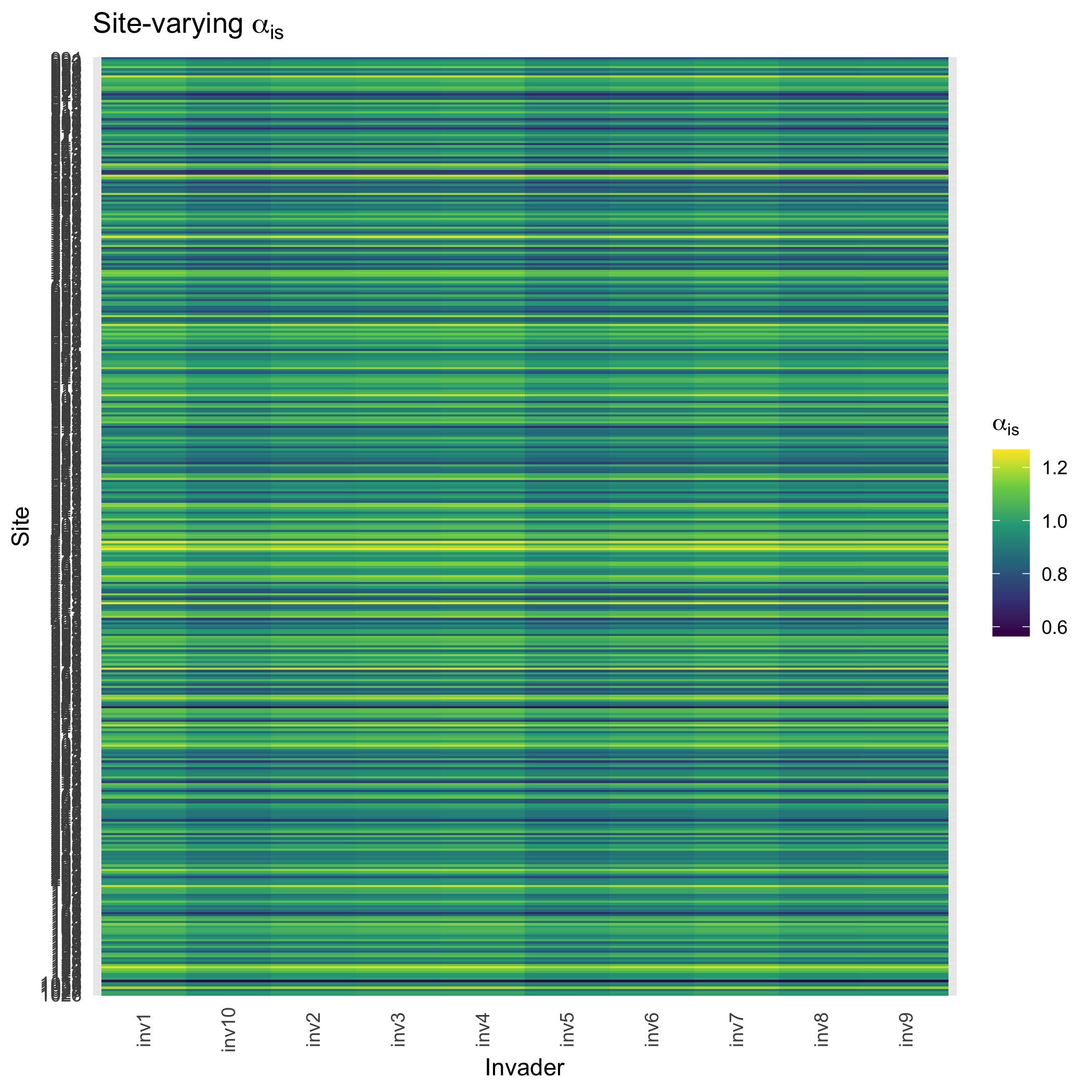
:chart_with_upwards_trend: Figure 11: The heatmaps show how sensitivity to crowding (
) varies across sites and invaders. Each column corresponds to an invader, each row to a site, and the colour scale represents the parameter value. Here, values are consistently positive but display subtle gradients across sites, indicating that some environments impose stronger penalties from trait overlap than others. This heterogeneity reflects local differences in how resident communities constrain invaders: higher (yellow-green) means stronger crowding effects, while lower values (blue-purple) suggest weaker suppression.
ggplot2::ggplot(abg_df, ggplot2::aes(invader, site, fill = Gamma_is)) + ggplot2::geom_tile() + ggplot2::scale_fill_viridis_c(name = expression(Gamma[is])) + ggplot2::labs(title = expression("Site-varying " * Gamma[is]), x = "Invader", y = "Site") + ggplot2::theme_minimal(base_size = 11) + ggplot2::theme(axis.text.x = ggplot2::element_text(angle = 90, vjust = 0.5))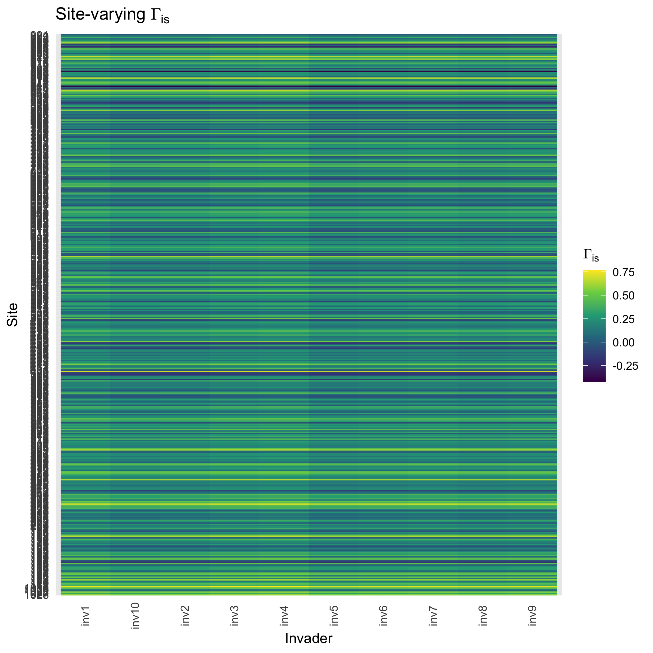
:chart_with_upwards_trend: Figure 12: The heatmaps show how sensitivity to abiotic scaling (
, second) varies across sites and invaders.Each column corresponds to an invader, each row to a site, and the colour scale represents the parameter value. Here, values describe how abiotic suitability scales for each invader—site combination. Most values fall near zero to moderate positive ranges, but some sites show locally elevated , highlighting environments where abiotic alignment disproportionately boosts invasion fitness.
:bar_chart: Together, the plots above confirm that invasion fitness is shaped by site-specific interactions: even with the same trait predictors, the balance between abiotic suitability and crowding penalties varies geographically. This heterogeneity is crucial for interpreting invasion outcomes, since invaders may thrive in sites where abiotic boosts outweigh crowding, while failing elsewhere despite similar trait distances.
:sparkles: Overall importance: These sensitivities are the coefficients that connect predictors to invasion fitness in flexible ways (constant, trait-varying, site-varying).
:bulb: Summary. You now have
Invader predictors
Section titled “Invader predictors ”predict_invaders() builds invader-side pillars on the resident scale using the residents GLMM, trait geometry, and resident moments.
:hourglass_flowing_sand: Step-by-step predict_invaders():
- Predicts invader
from fixed effects; - Standardises by resident site moments;
- Computes invader-resident distances and kernels to obtain
; - Standardises by resident moments;
- Broadcasts
to .
:zap: Run predict_invaders() to produce invader predictor matrices and tidy frames, aligning invaders directly to residents’ scales to avoid leakage.
# try(source("D:/Methods/R/myR_Packages/b-cubed-versions/invasimapr/R/predict_invaders.R"), silent = TRUE)# if (!exists("predict_invaders")) stop("predict_invaders() not found.")
fit = predict_invaders(fit, traits_inv)
# str(fit$invaders, 1)
r_is   = fit$invaders$r_isr_is_z = fit$invaders$r_is_zC_is   = fit$invaders$C_isC_is_z = fit$invaders$C_is_zS_is_z = fit$invaders$S_is_z
inv_predict_df = fit$invaders$dfsummary(inv_predict_df)#>       site        invader              r_link             r_z                 C_z#>  82     :  10   Length:4150        Min.   :-1.9422   Min.   :-8.447911   Min.   :-1.0035#>  83     :  10   Class :character   1st Qu.: 0.6978   1st Qu.:-0.830539   1st Qu.: 0.5128#>  84     :  10   Mode  :character   Median : 1.2211   Median : 0.136880   Median : 0.9441#>  117    :  10                      Mean   : 1.1506   Mean   :-0.008854   Mean   : 0.9597#>  118    :  10                      3rd Qu.: 1.6929   3rd Qu.: 0.993591   3rd Qu.: 1.3796#>  119    :  10                      Max.   : 3.6457   Max.   : 6.559607   Max.   : 3.3913#>  (Other):4090#>       S_z#>  Min.   :-1.5449#>  1st Qu.:-0.7173#>  Median :-0.1541#>  Mean   : 0.0000#>  3rd Qu.: 0.4529#>  Max.   : 5.6963#>
:bar_chart: Site maps of mean
stopifnot(exists("site_df"))
df_r_site = inv_predict_df |>  dplyr::group_by(site) |>  dplyr::mutate(mean_r_z = mean(r_z)) |>  dplyr::left_join(site_df, by = "site")
ggplot2::ggplot(df_r_site, ggplot2::aes(x, y, fill = mean_r_z)) +  ggplot2::geom_tile() +  ggplot2::scale_fill_gradient2(name = expression(Mean~r^{(z)}), midpoint = 0) +  ggplot2::labs(title = expression("Abiotic suitability " * r^{(z)} * " (site mean across invaders)"),                x = "x", y = "y") +  ggplot2::theme_minimal() +  ggplot2::geom_sf(data = rsa, inherit.aes = FALSE, fill = NA, color = "black", size = 0.3)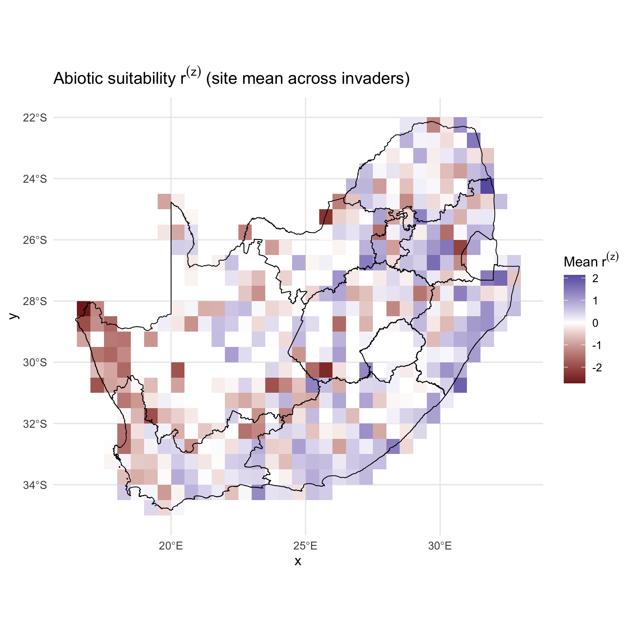
:chart_with_upwards_trend: Figure 13: This map summarises how Abiotic Suitability (
) co-varies across space, averaged over all invaders. Here, the colours reflect the mean abiotic suitability that invaders experience per site. Warmer red tones indicate lower or even negative suitability, while cooler blue tones show higher suitability. The spatial gradients capture regions where abiotic conditions consistently favour or hinder invasion potential.
stopifnot(exists("site_df"))
df_C_site = inv_predict_df |>  dplyr::group_by(site) |>  dplyr::mutate(mean_C_z = mean(C_z)) |>  dplyr::left_join(site_df, by = "site")
ggplot2::ggplot(df_C_site, ggplot2::aes(x, y, fill = mean_C_z)) +  ggplot2::geom_tile() +  ggplot2::scale_fill_viridis_c(name = expression(Mean~C^{(z)}), direction = 1) +  ggplot2::labs(    title = expression("Trait-similar crowding " * C^{(z)} * " (site mean across invaders)"),    x = "x", y = "y"  ) +  ggplot2::theme_minimal() +  ggplot2::geom_sf(data = rsa, inherit.aes = FALSE, fill = NA, color = "black", size = 0.3)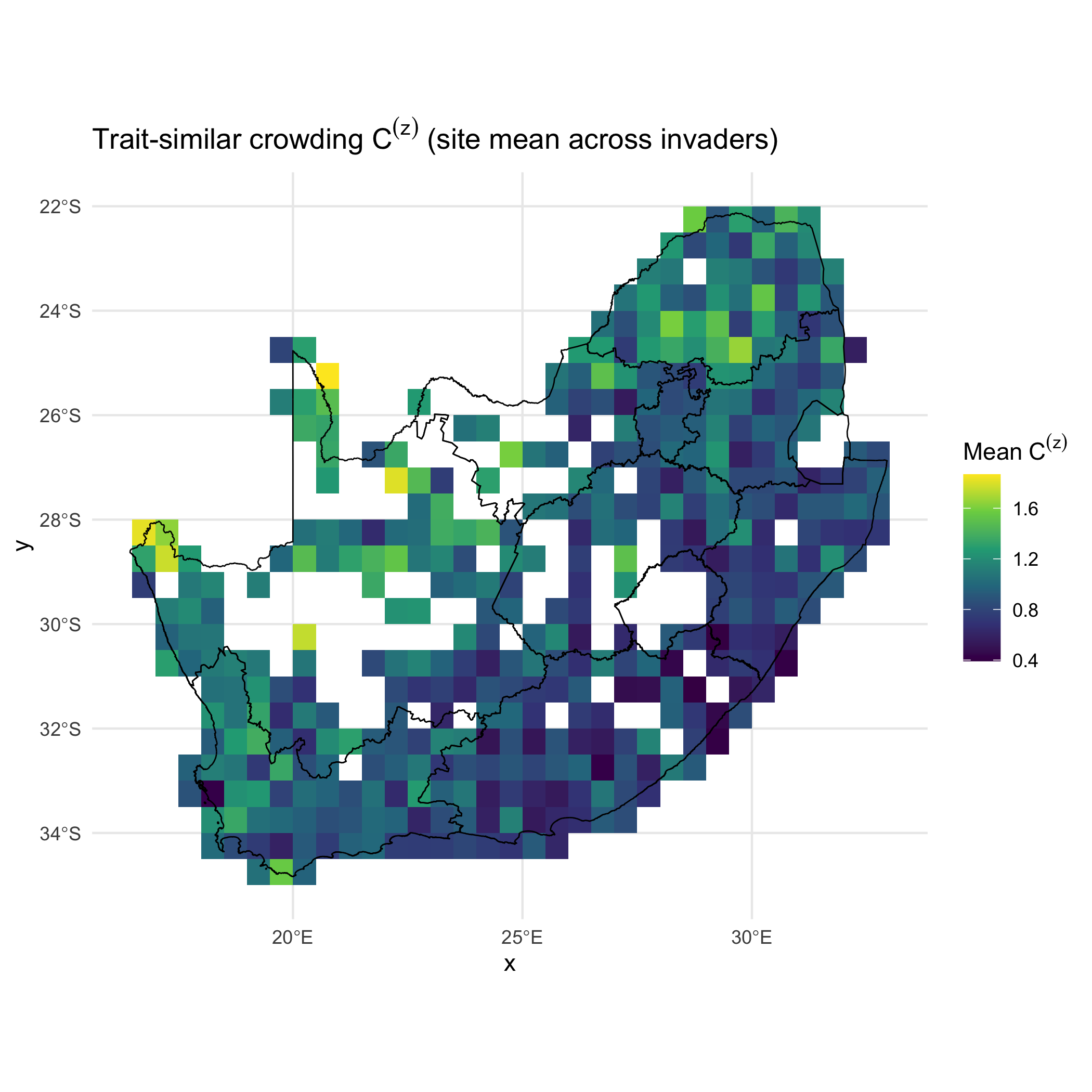
:chart_with_upwards_trend: Figure 14: This map summarises how Trait-similar Crowding (
) or biotic pressure co-varies across space, averaged over all invaders. Here, the colours represent the average intensity of biotic pressure from resident communities, scaled by trait similarity. Higher values (yellow-green) highlight areas where residents are more functionally similar to potential invaders, thus exerting stronger competitive exclusion. Lower values (blue-purple) identify sites where invaders may face less trait-overlap pressure.
:bar_chart: Together, these maps provide a spatial lens on the trade-off between abiotic opportunity and biotic resistance: invasion is more likely where
:sparkles: Overall importance: Invader predictors are now on the same within-site scales as residents, enabling apples-to-apples fitness calculations.
:bulb: Summary. You now have
Invasion fitness (
Section titled “Invasion fitness () and establishment probability ()”predict_establishment() combines invader predictors with sensitivities under a set of options (A-E) and maps
:hourglass_flowing_sand: Step-by-step predict_establishment():
- Selects coefficients (constant, trait-varying, site-varying),
- optionally calibrates a resident baseline,
- computes
, and transforms to . - Finally, it returns matrices plus tidy long frames and optional plots.
:zap: Run predict_establishment() to produce
library(ggplot2)  # ensures waiver() exists# try(source("D:/Methods/R/myR_Packages/b-cubed-versions/invasimapr/R/predict_establishment.R"), silent = TRUE)# if (!exists("predict_establishment")) stop("predict_establishment() not found.")
fit = predict_establishment(  fit,  option         = "A",          # try "A"..."E"  prob_method    = "hard",       # "probit", "logit", or "hard"  prob_scale     = list(sigma = 1),  calibrate_kappa = TRUE,  boundary_sf    = rsa)
str(fit,1)#> List of 11#>  $ inputs       :List of 13#>  $ meta         :List of 7#>  $ inputs_std   :List of 2#>  $ traits       :List of 10#>  $ crowding     :List of 5#>  $ model        :List of 7#>  $ residents    :List of 16#>  $ sensitivities:List of 26#>  $ invaders     :List of 6#>  $ fitness      :List of 7#>  $ prob         :List of 7#>  - attr(*, "class")= chr [1:2] "invasimapr_fit" "list"# str(fit$fitness, 1)# str(fit$prob, 1)
lambda_is = fit$fitness$lambda_isp_is      = fit$prob$p_is# fit_lambda = fit$fitness$lambda_long
:bar_chart: Overall mean
if (!is.null(fit$prob$plots$heatmap)) fit$prob$plots$heatmap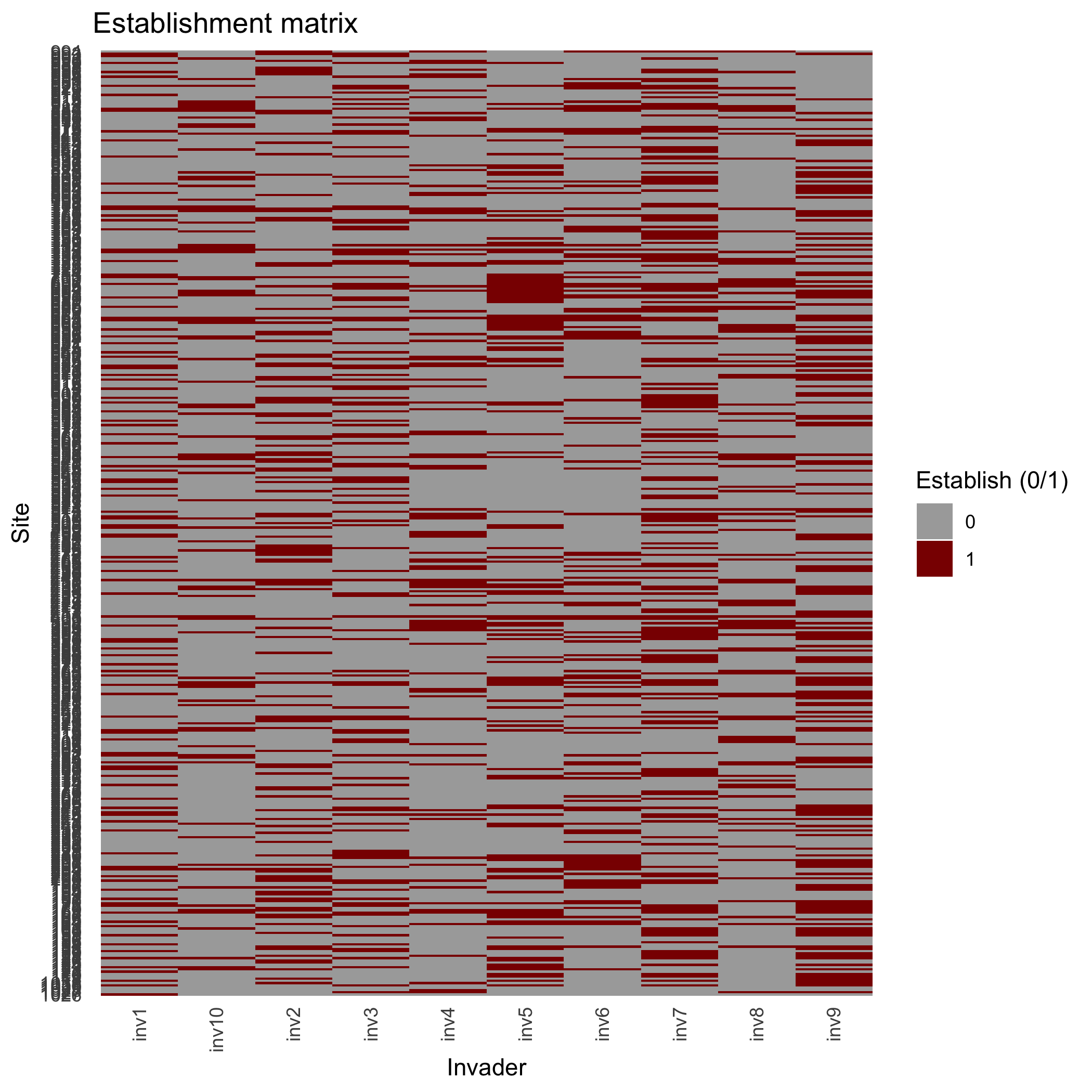
:chart_with_upwards_trend: Figure 15: This figure illustrates the spatial and invader-specific structure of establishment likelihood. Rows correspond to sites and columns to invaders, with cells showing binary establishment outcomes. The sparse but structured pattern of yellow cells (successful establishment) indicates that invasion is not uniform but instead constrained by both species identity and site context.
# str(fit$prob$plots, 1)if (!is.null(fit$prob$plots$site_mean)) fit$prob$plots$site_mean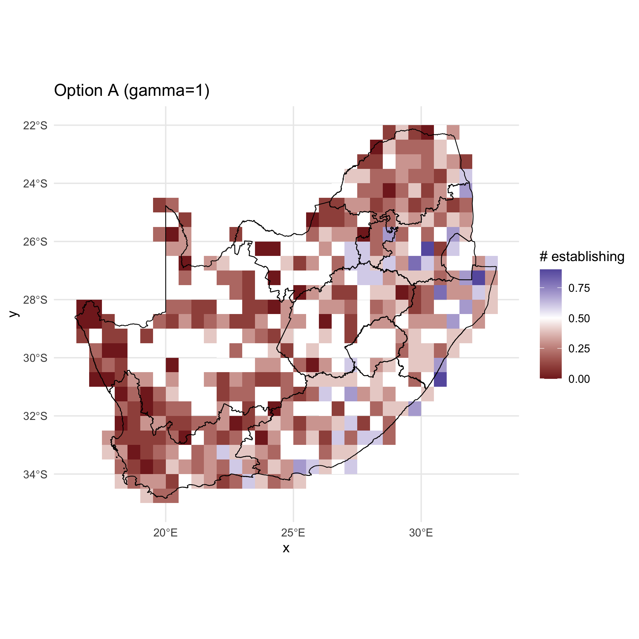
:chart_with_upwards_trend: Figure 16: Spatial pattern of establishment under Option A (
= 1). Tiles show the number/proportion of species establishing per grid cell (“# establishing”), from low (brown) to high (blue), over South Africa’s boundaries.
# str(fit$prob$plots, 1)if (!is.null(fit$prob$plots$invader_mean)) fit$prob$plots$invader_mean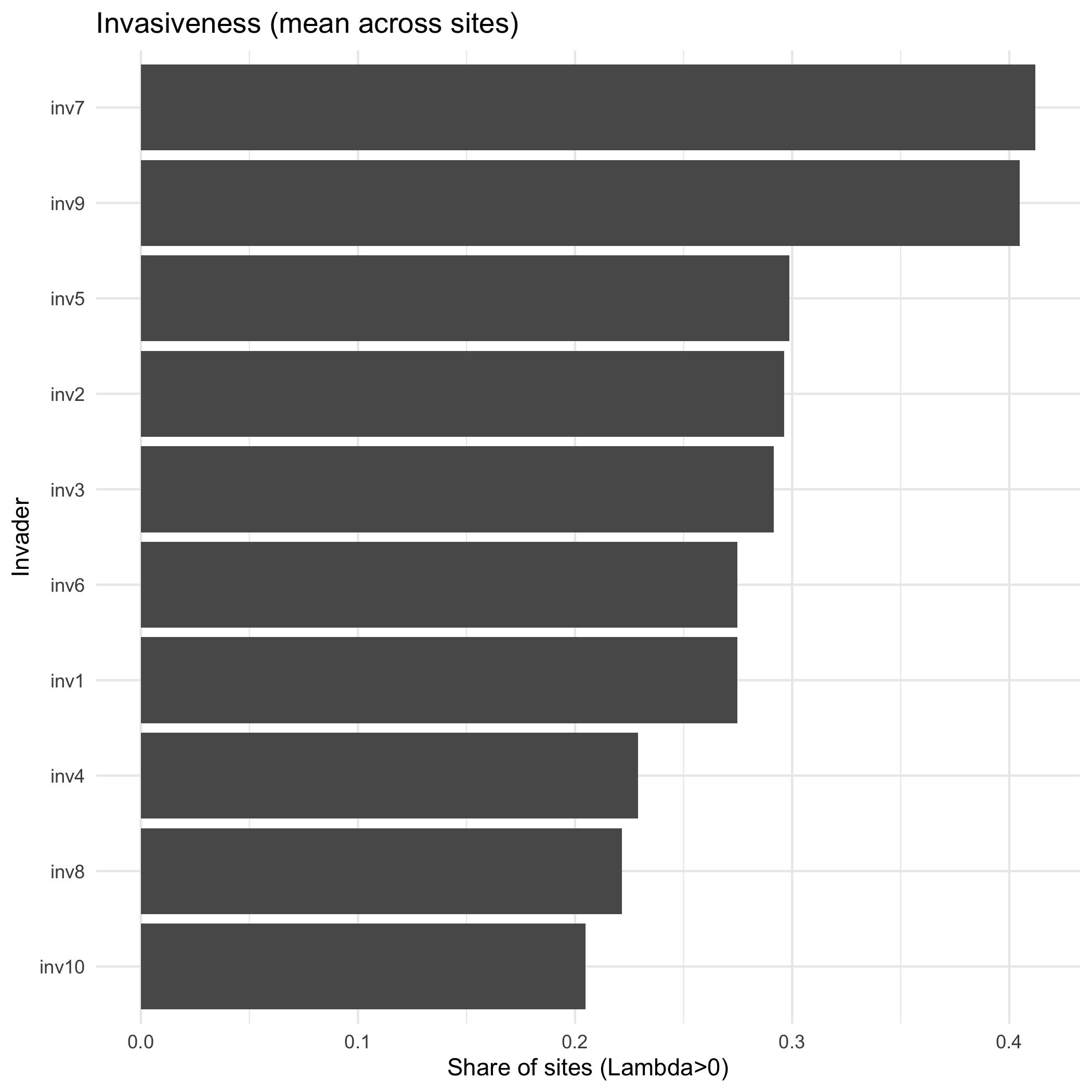
:chart_with_upwards_trend: Figure 17: Invasiveness ranking by invader. Bars show the mean fraction of sites where intrinsic growth is positive (
> 0) for each invader, averaged across all sites and ordered from highest (more invasive; e.g., inv7, inv9) to lowest (e.g., inv10).
fitness_df = fit$fitness$lambda_long |> dplyr::group_by(site, x, y, option) |> dplyr::summarise(lambda_mean = mean(lambda, na.rm = TRUE), .groups = "drop")ggplot2::ggplot(fitness_df, ggplot2::aes(x, y, fill = lambda_mean)) + ggplot2::geom_tile() + ggplot2::scale_fill_gradient2(name = "Mean lambda", midpoint = -1.707) + ggplot2::geom_sf(data = rsa, inherit.aes = FALSE, fill = NA, color = "black", size = 0.3) + ggplot2::labs(title = fitness_df$option, x = "x", y = "y") + ggplot2::theme_minimal()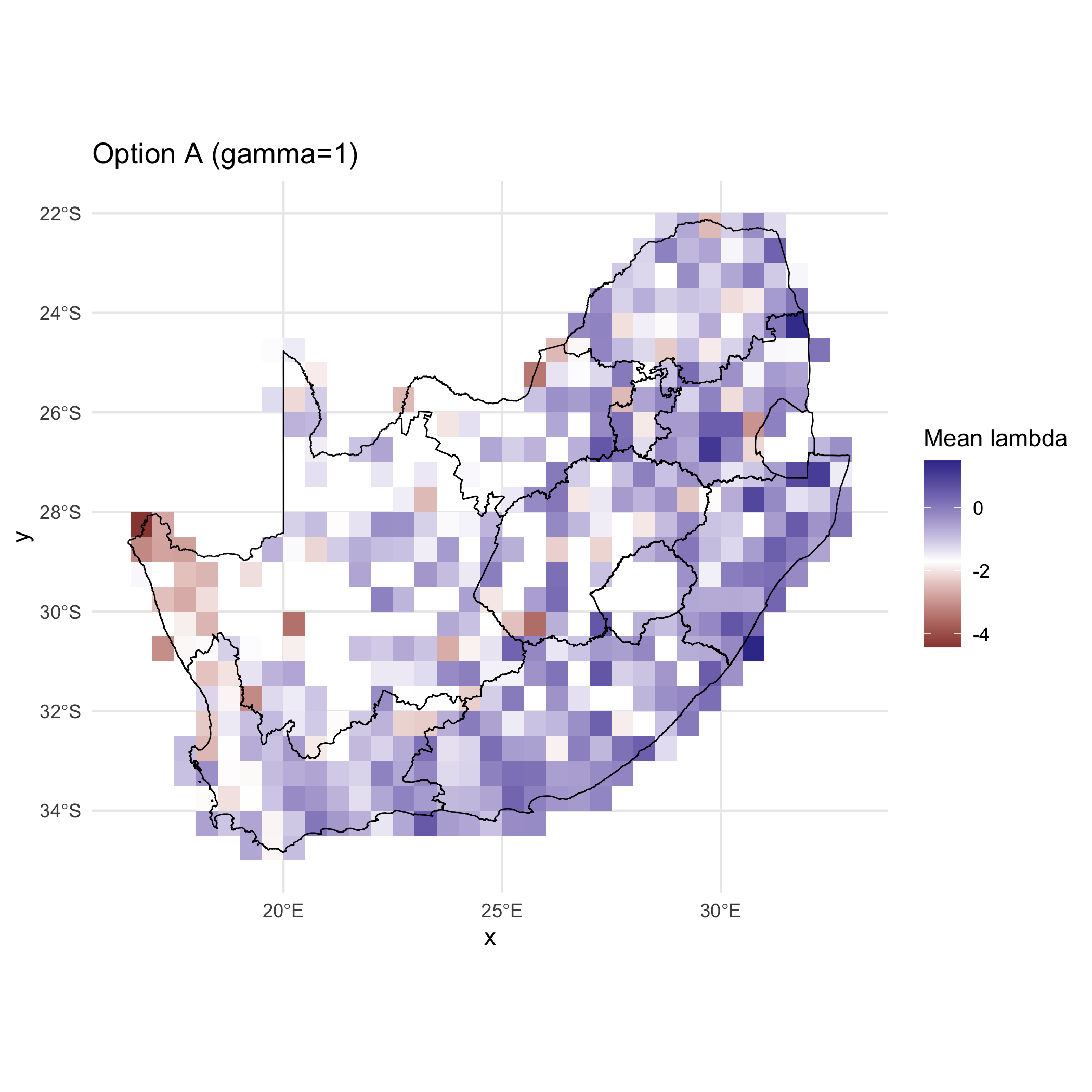
:chart_with_upwards_trend: Figure 18: This figures illustrates the spatial and invader-specific structure of establishment likelihood. Mean
is mapped with colours reflecting the site-level mean fitness ( ) of invaders under option A ( ), summarising overall openness to establishment. Negative values (brown) dominate, showing that most sites are generally resistant, while scattered blue patches identify hotspots where conditions are sufficiently favourable for invader persistence.
:bar_chart: Together, the heatmap and map highlight the joint filtering effects of species identity and geography: while few invaders succeed broadly, specific site—species combinations align to permit establishment, with spatial clustering of higher openness revealing invasion-prone regions.
:sparkles: Overall importance: These outputs translate biotic and abiotic structure into explicit establishment surfaces, ready for summary and decision-support.
:bulb: Summary. You now have
Summaries: species, traits, and sites
Section titled “Summaries: species, traits, and sites”summarise_results() distils the full
:hourglass_flowing_sand: Step-by-step summarise_results():
- Computes
and (hard or probabilistic), - Ranks invaders and sites,
- Quantifies trait-fitness relationships, and
- Returns plots (e.g. maps, heatmaps, lollipop plots) and summary tables.
:zap: Run summarise_results() to produce decision-ready summaries and figures linked back to the same predictors and trait geometry.
# try(source("D:/Methods/R/myR_Packages/b-cubed-versions/invasimapr/R/summarise_results.R"), silent = TRUE)# if (!exists("summarise_results")) stop("summarise_results() not found.")
fit = summarise_results(  fit,  use_probabilistic = TRUE,  make_plots        = TRUE,  boundary_sf       = rsa)
str(fit, 1)#> List of 12#>  $ inputs       :List of 13#>  $ meta         :List of 7#>  $ inputs_std   :List of 2#>  $ traits       :List of 10#>  $ crowding     :List of 5#>  $ model        :List of 7#>  $ residents    :List of 16#>  $ sensitivities:List of 26#>  $ invaders     :List of 6#>  $ fitness      :List of 7#>  $ prob         :List of 7#>  $ summary      :List of 6#>  - attr(*, "class")= chr [1:2] "invasimapr_fit" "list"str(fit$summary, 1)#> List of 6#>  $ species       : tibble [10 × 5] (S3: tbl_df/tbl/data.frame)#>  $ site          : tibble [415 × 9] (S3: tbl_df/tbl/data.frame)#>  $ trait_effects : tibble [20 × 7] (S3: tbl_df/tbl/data.frame)#>  $ establish_long: tibble [4,150 × 8] (S3: tbl_df/tbl/data.frame)#>  $ plots         :List of 4#>  $ meta          :List of 3# head(dplyr::arrange(fit$summary$species, dplyr::desc(V_i)), 10)# head(dplyr::arrange(fit$summary$site,    dplyr::desc(total_expected %||% n_est)), 10)# fit$summary$trait_effects
:bar_chart: Species & trait invasiveness and site invasibility maps
if (!is.null(fit$summary$plots$invader_rank)) fit$summary$plots$invader_rank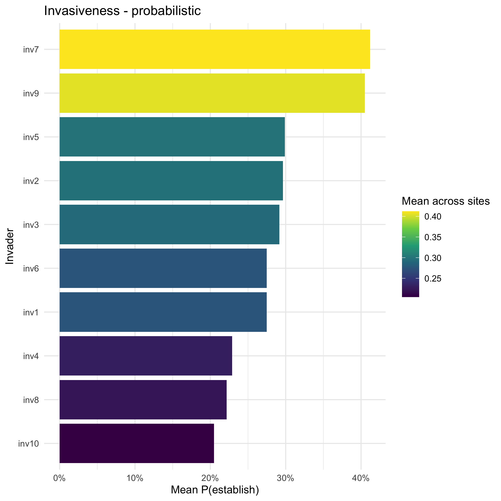
:chart_with_upwards_trend: Figure 19: Invasiveness - probabilistic view where bars show the mean probability of establishment across sites for each invader. A steep drop from the top few taxa to the remainder indicates a short “high-risk list”: a small subset of invaders (e.g., inv6—inv7) are consistently more likely to establish, while others rarely exceed low single-digit probabilities. This ranking is useful for triage and horizon scanning.
if (!is.null(fit$summary$plots$site_map)) fit$summary$plots$site_map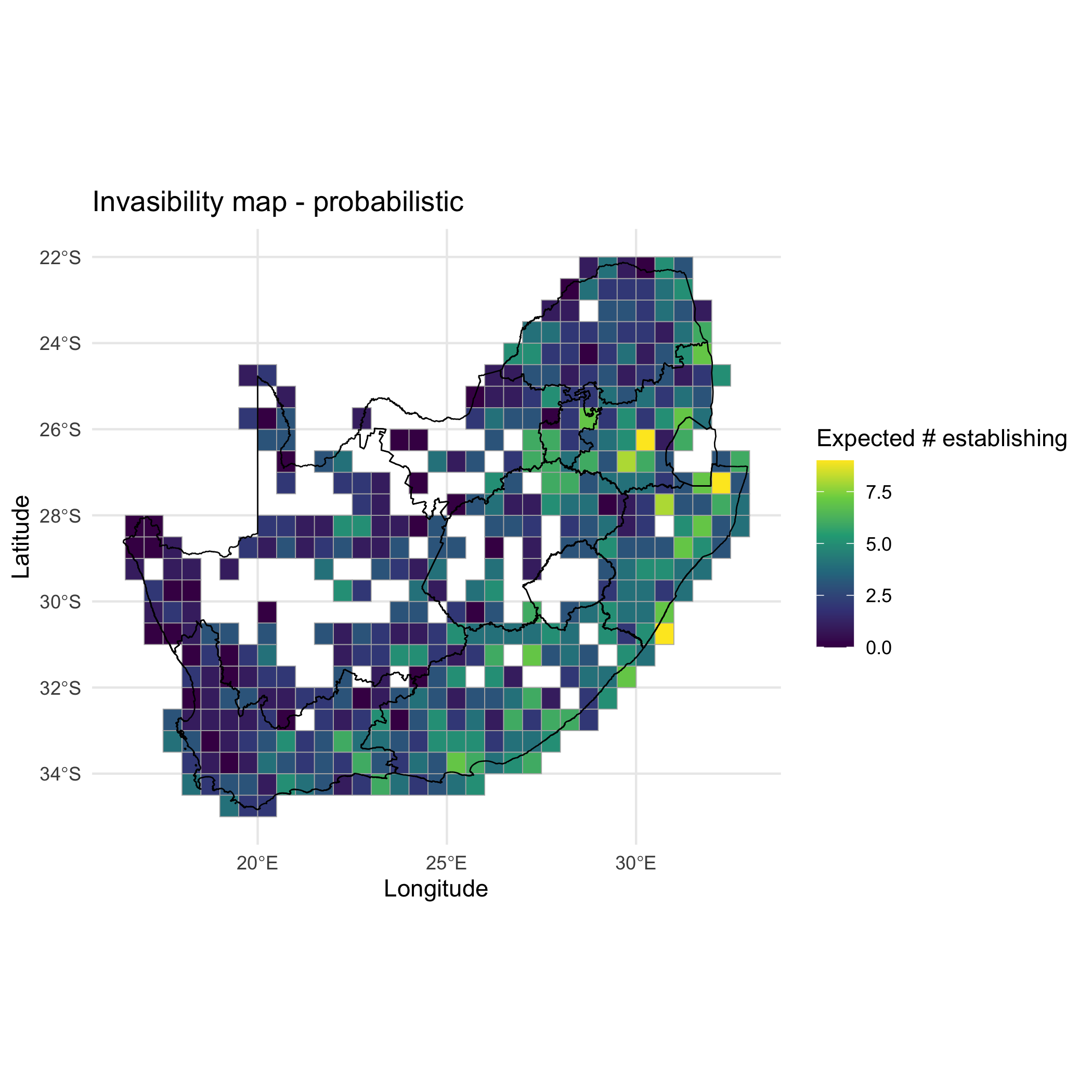
:chart_with_upwards_trend: Figure 20: Invasibility map - probabilistic view where colours map the expected number of establishing invaders per site (sum of probabilities), highlighting geographic hotspots of openness. Most of the country remains resistant (dark tones), but clusters of higher expected establishment emerge along specific regions and borders, suggesting where surveillance or rapid response capacity would yield the greatest return.
if (!is.null(fit$summary$plots$heatmap)) fit$summary$plots$heatmap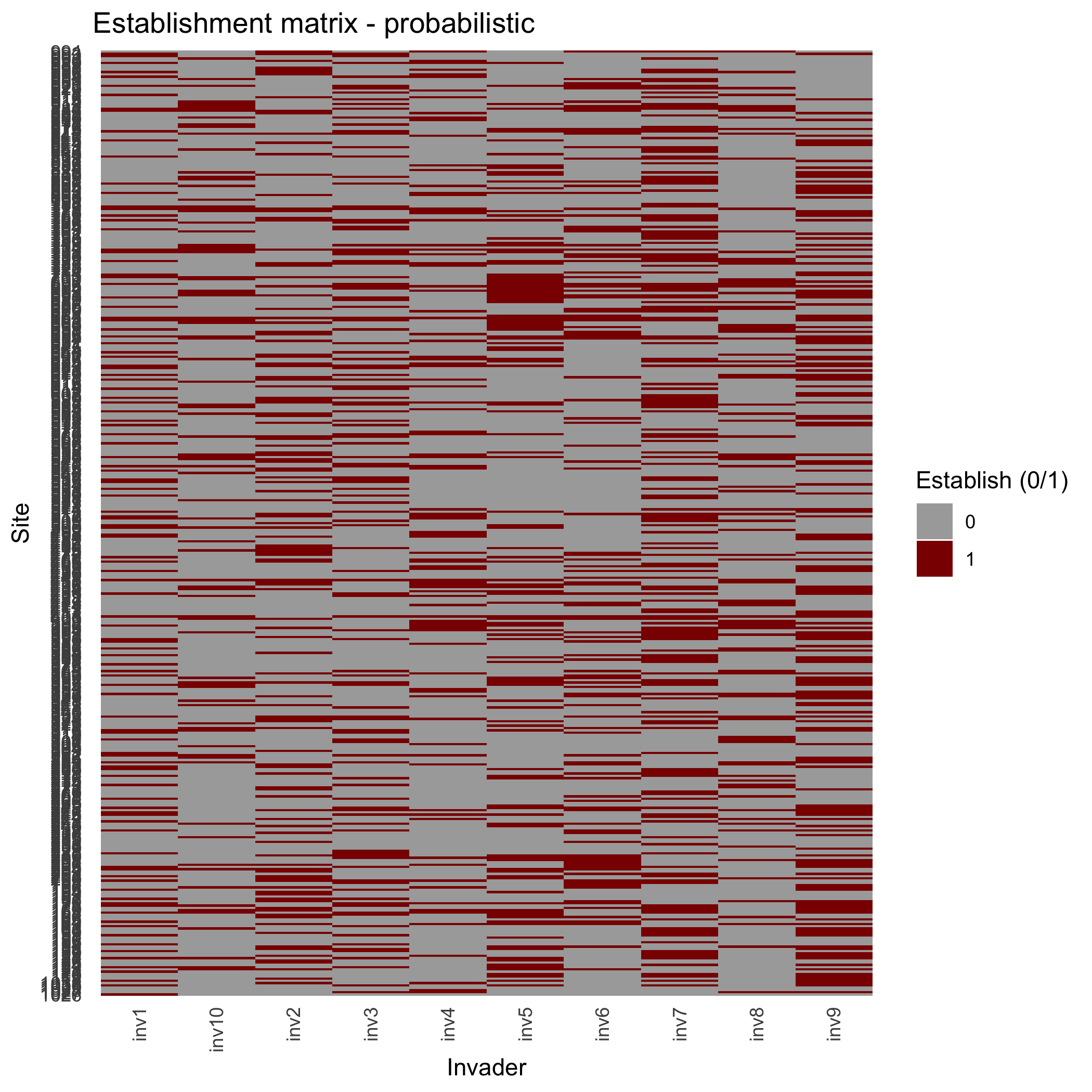
:chart_with_upwards_trend: Figure 21: Establishment matrix with binary establishment outcomes from the probabilistic model shown across sites and invaders. Rows are sites, columns are invaders; tiles show establishment (1, red) vs non-establishment (0, grey), illustrating heterogeneity among invaders and among sites.
if (!is.null(fit$summary$plots$trait_effects)) fit$summary$plots$trait_effects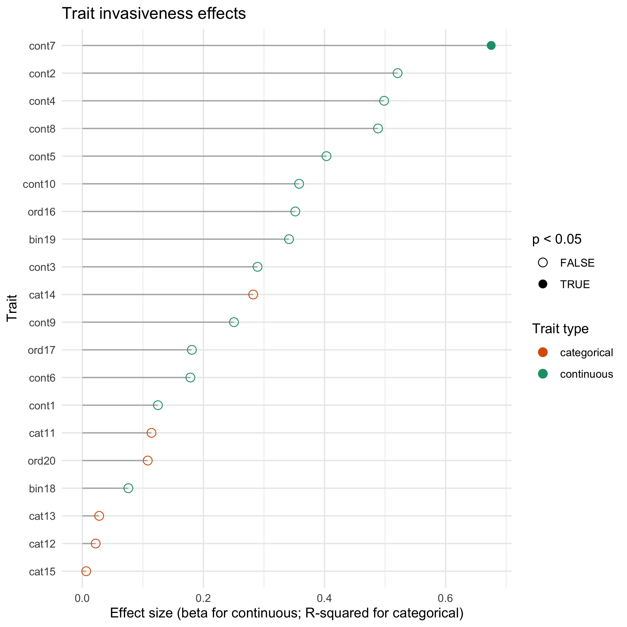
:chart_with_upwards_trend: Figure 22: Trait invasiveness effects view with a lollipop plot ranks traits by their association with mean establishment probability (|β| for continuous traits; ANOVA
for categorical/ordinal). A small set of continuous traits dominate the signal (right side, several with ), implying that functional axes captured by those traits systematically raise or lower invasion success. Categorical/ordinal traits contribute more modestly, pointing to ecologically relevant but weaker thresholds or syndromes.
:bar_chart: A few invaders and a few trait axes drive most risk, and their success concentrates in identifiable regions. This combination, who, why, and where, provides a clear basis for prioritising monitoring, pathway management, and site-level mitigation. Ranked bars highlight consistently risky invaders; site maps show hotspots of openness; heatmaps reveal joint structure; trait lollipops identify functional correlates.
:sparkles: Overall importance: These summaries compress high-dimensional predictions into interpretable priorities for surveillance and management.
:bulb: Summary. You now have species ranks
# # 1) Count of all val==1 by site (heatmap)# site_counts = fit$summary$establish_long |>#   group_by(site, x, y) |>#   summarise(n_val1 = sum(val == 1L, na.rm = TRUE),#             p_val1 = (sum(val == 1L, na.rm = TRUE)/length(unique(fit$summary$establish_long$invader)))*100, .groups = "drop")# head(site_counts)## p_count = ggplot2::ggplot(site_counts, ggplot2::aes(x, y, fill = n_val1)) +#   ggplot2::geom_tile() +#   ggplot2::coord_equal() +#   ggplot2::scale_fill_viridis_c(name = "# invaders with val = 1", option = "C") +#   ggplot2::geom_sf(data = rsa, inherit.aes = FALSE, fill = NA, color = "black", size = 0.35) +#   ggplot2::labs(title = "Count of val = 1 by site", x = "Longitude", y = "Latitude") +#   ggplot2::theme_minimal(base_size = 12)# print(p_count)
# p_prop = ggplot2::ggplot(site_counts, ggplot2::aes(x, y, fill = p_val1)) +#   ggplot2::geom_tile() +#   ggplot2::coord_equal() +#   ggplot2::scale_fill_viridis_c(name = "% invaders with val = 1", option = "C") +#   ggplot2::geom_sf(data = rsa, inherit.aes = FALSE, fill = NA, color = "black", size = 0.35) +#   ggplot2::labs(title = "% of val = 1 by site", x = "Longitude", y = "Latitude") +#   ggplot2::theme_minimal(base_size = 12)# print(p_prop)
# 2) Separate maps per invader: val=1 red, val=0 dark greydf_inv = fit$summary$establish_long |>  dplyr::mutate(val_f = factor(val, levels = c(0, 1)))
p_facets = ggplot2::ggplot(df_inv, ggplot2::aes(x, y, fill = val_f)) +  ggplot2::geom_tile() +  ggplot2::coord_equal() +  ggplot2::scale_fill_manual(    values = c(`0` = "grey20", `1` = "#d7301f"),    labels = c(`0` = "0", `1` = "1"),    name   = "val"  ) +  ggplot2::facet_wrap(~ invader, ncol = 5) +  ggplot2::geom_sf(data = rsa, inherit.aes = FALSE, fill = NA, color = "black", size = 0.35) +  labs(title = "Per-invader maps (val = 1 in red, val = 0 in dark grey)",       x = "Longitude", y = "Latitude") +  ggplot2::theme_minimal(base_size = 12) +  ggplot2::theme(axis.text.x = ggplot2::element_blank(),        axis.text.y = ggplot2::element_blank())print(p_facets)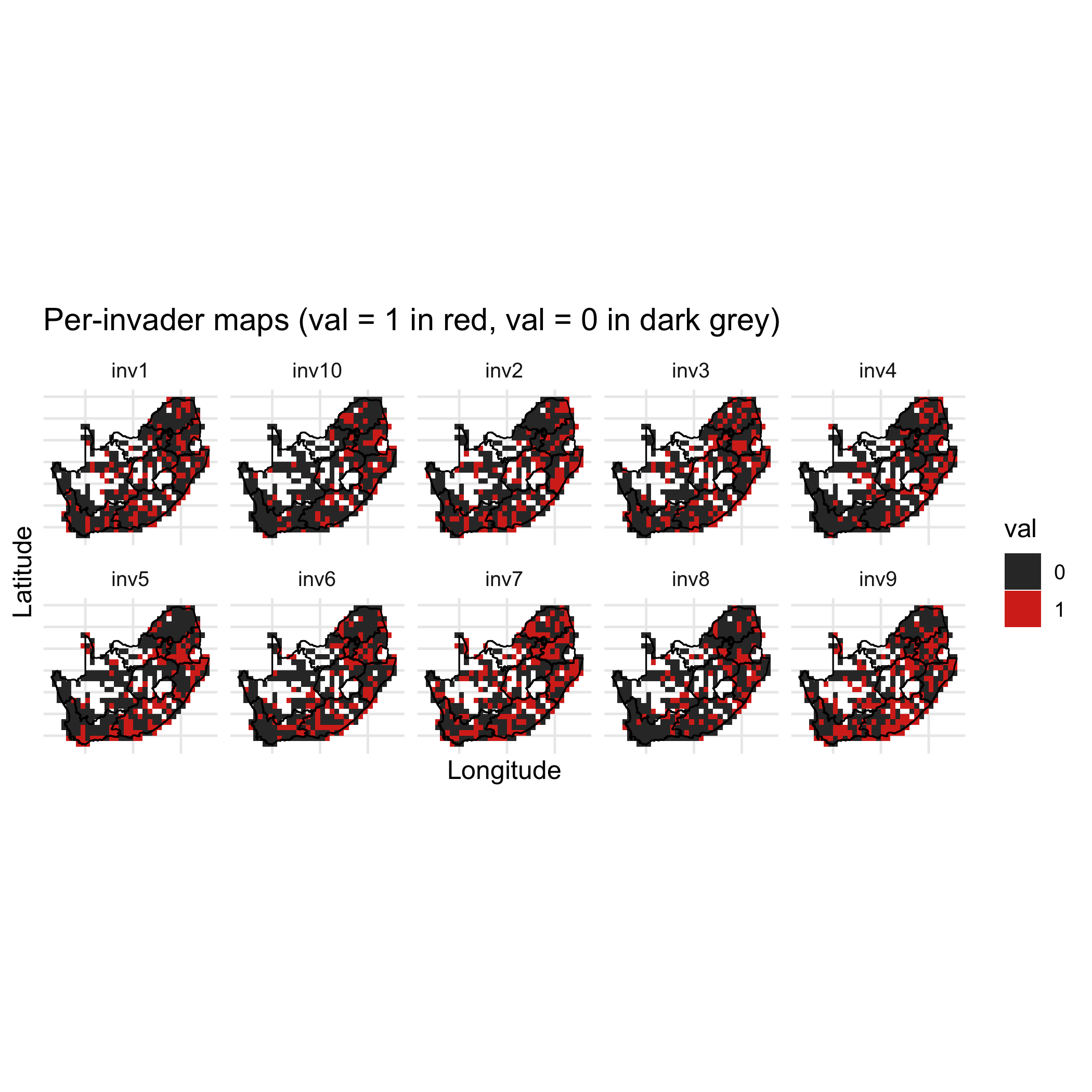
:chart_with_upwards_trend: Figure 23: Per-invader maps of binary establishment across South Africa. Each panel is one invader; red cells indicate establishment (1) and dark grey non-establishment (0). Common grid and coastline enable direct comparison of spatial patterns among invaders.
Common pitfalls & quick fixes
Section titled “Common pitfalls & quick fixes”Final guardrails for robust runs and reproducibility.
- Name alignment. All site-indexed matrices use identical rownames; community columns match trait rownames.
- Hull stability. Use ≥3 residents; otherwise centrality/hull diagnostics may be skipped.
- Standardisation leakage. Scale invaders using resident moments only.
- Prediction scale. Use fixed-effects predictions (
re.form = NA) for both residents and invaders. - Saturation slopes. Do not add
(0 + S_z || site);S_zhas no within-site variation.
Session information
Section titled “Session information”sessionInfo()#> R version 4.5.3 (2026-03-11)#> Platform: aarch64-apple-darwin20#> Running under: macOS Tahoe 26.5#>#> Matrix products: default#> BLAS: /System/Library/Frameworks/Accelerate.framework/Versions/A/Frameworks/vecLib.framework/Versions/A/libBLAS.dylib#> LAPACK: /Library/Frameworks/R.framework/Versions/4.5-arm64/Resources/lib/libRlapack.dylib; LAPACK version 3.12.1#>#> locale:#> [1] en_US.UTF-8/en_US.UTF-8/en_US.UTF-8/C/en_US.UTF-8/en_US.UTF-8#>#> time zone: Europe/Brussels#> tzcode source: internal#>#> attached base packages:#> [1] stats graphics grDevices utils datasets methods base#>#> other attached packages:#> [1] fs_2.1.0 rmarkdown_2.31 ggplot2_4.0.3 invasimapr_0.2.0 b3doc_0.3.0.9000#> [6] here_1.0.2 purrr_1.2.2 yaml_2.3.12#>#> loaded via a namespace (and not attached):#> [1] splines_4.5.3 later_1.4.8 fields_17.3 tibble_3.3.1#> [5] R.oo_1.27.1 hardhat_1.4.3 pROC_1.19.0.1 rpart_4.1.24#> [9] factoextra_2.0.0 lifecycle_1.0.5 rstatix_0.7.2 Rdpack_2.6.4#> [13] sf_1.1-1 rprojroot_2.1.1 globals_0.19.1 processx_3.9.0#> [17] lattice_0.22-9 MASS_7.3-65 backports_1.5.1 dendextend_1.19.1#> [21] NbClust_3.0.1 magrittr_2.0.5 otel_0.2.0 spam_2.11-1#> [25] sp_2.2-1 pbapply_1.7-4 chromote_0.5.1 DBI_1.3.0#> [29] minqa_1.2.8 RColorBrewer_1.1-3 lubridate_1.9.5 abind_1.4-8#> [33] multcomp_1.4-30 maps_3.4.3 rvest_1.0.4 glmmTMB_1.1.14#> [37] R.utils_2.13.0 nnet_7.3-20 TH.data_1.1-3 rappdirs_0.3.4#> [41] sandwich_3.1-1 ipred_0.9-15 lava_1.9.1 ggrepel_0.9.8#> [45] listenv_0.10.1 terra_1.9-34 pheatmap_1.0.13 vegan_2.7-1#> [49] units_1.0-1 parallelly_1.47.0 permute_0.9-10 codetools_0.2-20#> [53] xml2_1.6.0 tidyselect_1.2.1 dissmapr_0.2.0 clValid_0.7#> [57] farver_2.1.2 lme4_2.0-1 viridis_0.6.5 matrixStats_1.5.0#> [61] stats4_4.5.3 jsonlite_2.0.0 caret_7.0-1 e1071_1.7-17#> [65] Formula_1.2-5 survival_3.8-6 iterators_1.0.14 emmeans_2.0.3#> [69] foreach_1.5.2 geodata_0.6-9 tools_4.5.3 stringdist_0.9.15#> [73] pak_0.10.0 Rcpp_1.1.1-1.1 glue_1.8.1 prodlim_2026.03.11#> [77] gridExtra_2.3 xfun_0.59 mgcv_1.9-4 websocket_1.4.4#> [81] dplyr_1.2.1 scam_1.2-22 withr_3.0.3 numDeriv_2016.8-1.1#> [85] fastmap_1.2.0 boot_1.3-32 entropy_1.3.2 callr_3.8.0#> [89] digest_0.6.39 timechange_0.4.0 R6_2.6.1 estimability_1.5.1#> [93] wk_0.9.5 fuzzyjoin_0.1.8 dichromat_2.0-0.1 R.methodsS3_1.8.2#> [97] utf8_1.2.6 tidyr_1.3.2 generics_0.1.4 data.table_1.18.4#> [101] recipes_1.3.1 class_7.3-23 httr_1.4.8 ModelMetrics_1.2.2.2#> [105] pkgconfig_2.0.3 gtable_0.3.6 timeDate_4041.110 rsconnect_1.5.0#> [109] S7_0.2.2 selectr_0.5-1 htmltools_0.5.9 carData_3.0-6#> [113] dotCall64_1.2 TMB_1.9.17 scales_1.4.0 gower_1.0.2#> [117] reformulas_0.4.4 corrplot_0.95 knitr_1.51 rstudioapi_0.17.1#> [121] geosphere_1.6-8 reshape2_1.4.5 coda_0.19-4.1 nlme_3.1-169#> [125] curl_7.1.0 nloptr_2.2.1 zetadiv_1.3.0 proxy_0.4-29#> [129] zoo_1.8-15 stringr_1.6.0 KernSmooth_2.23-26 parallel_4.5.3#> [133] s2_1.1.11 pillar_1.11.1 grid_4.5.3 vctrs_0.7.3#> [137] ggpubr_0.6.3 promises_1.5.0 car_3.1-5 xtable_1.8-8#> [141] cluster_2.1.8.2 evaluate_1.0.5 magick_2.9.1 mvtnorm_1.4-1#> [145] cli_3.6.6 compiler_4.5.3 rlang_1.2.0 ggsignif_0.6.4#> [149] future.apply_1.20.2 labeling_0.4.3 mclust_6.1.2 classInt_0.4-11#> [153] ps_1.9.3 forcats_1.0.1 plyr_1.8.9 stringi_1.8.7#> [157] viridisLite_0.4.3 Matrix_1.7-5 patchwork_1.3.2 future_1.70.0#> [161] rbibutils_2.3 broom_1.0.13